NVIDIA Newton Physics: GPU-Accelerated Simulation for Physical AI
Overview
Today I attended an NVIDIA workshop on Newton Physics - their new open-source GPU-accelerated physics simulation engine designed specifically for Physical AI development. The workshop was presented by Ninad Madhab from NVIDIA and covered the full stack from world foundation models to hands-on simulation.
- Date: December 20, 2025
- Duration: ~2 hours
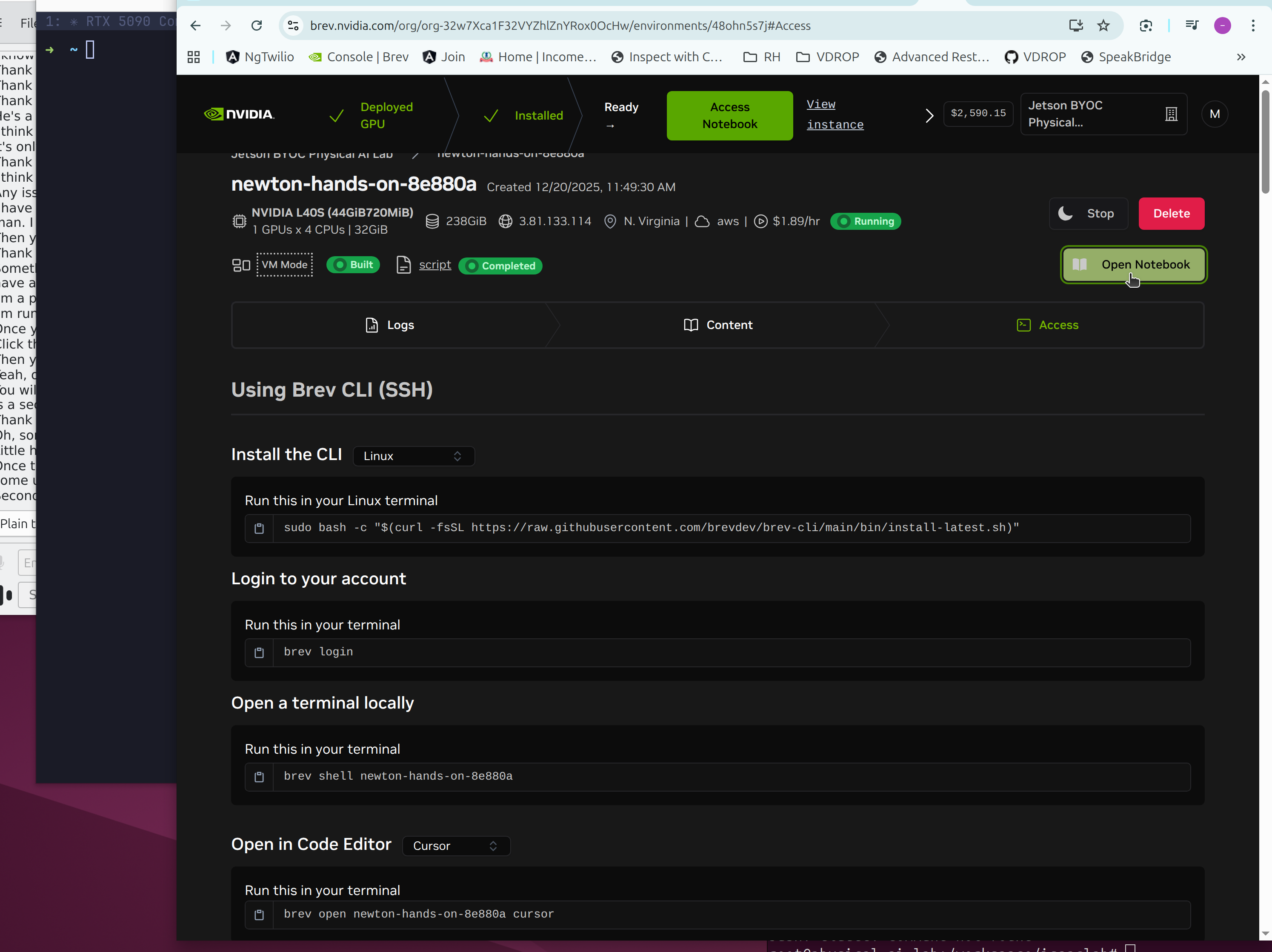
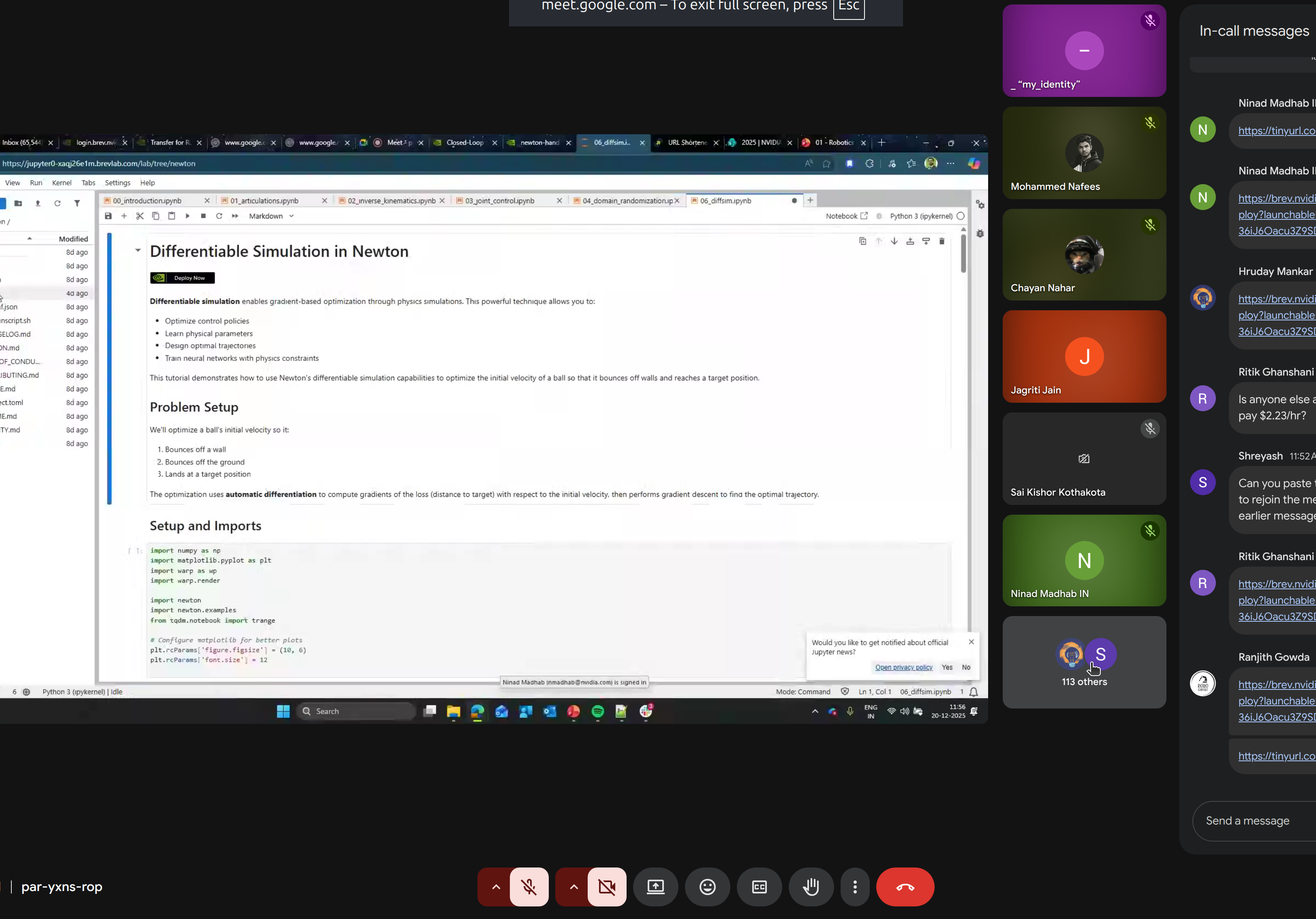
- Format: Presentation + Hands-on Lab (Brev.dev cloud)
- Presenter: Ninad Madhab, NVIDIA
The Physical AI Stack
NVIDIA’s vision for Physical AI involves multiple layers working together.
1. Cosmos World Foundation Models
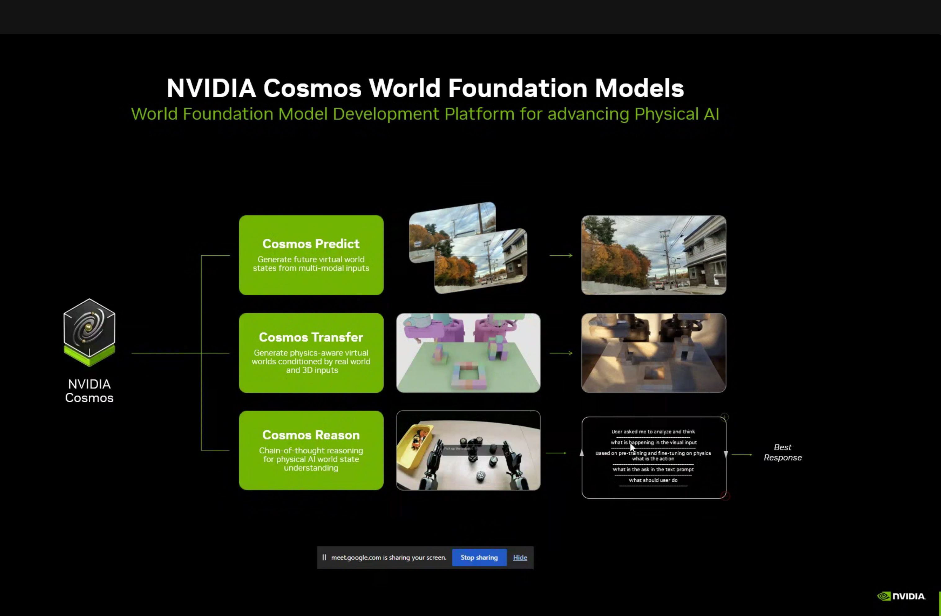
NVIDIA Cosmos is a platform for developing world foundation models that understand and can predict physical world behavior:
| Component | Purpose |
|---|---|
| Cosmos Predict | Generate future virtual world states from multi-modal inputs |
| Cosmos Transfer | Generate physics-aware virtual worlds conditioned by real world and 3D inputs |
| Cosmos Reason | Chain-of-thought reasoning for physical AI world state understanding |
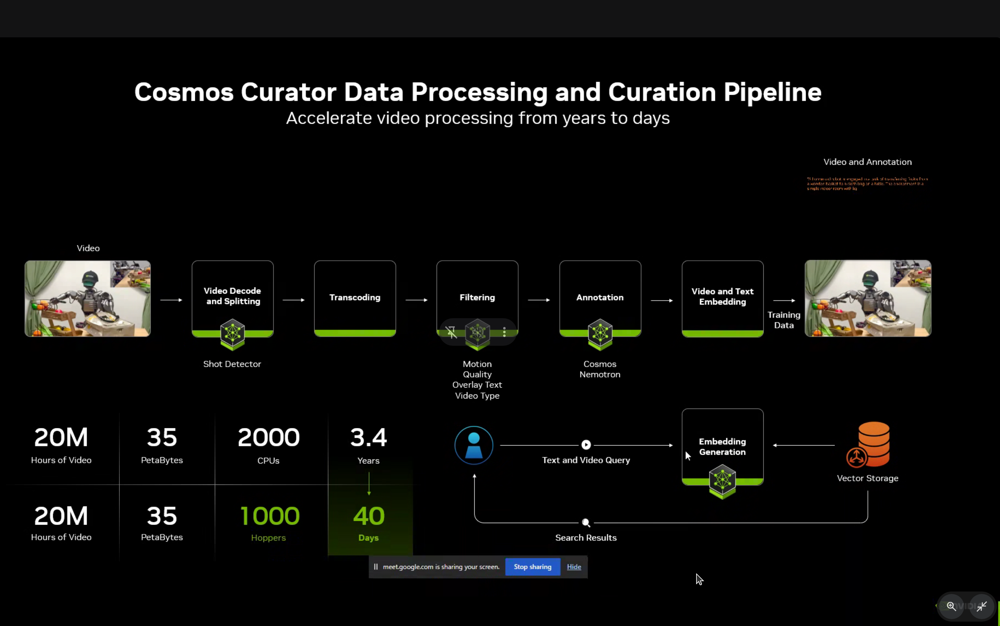
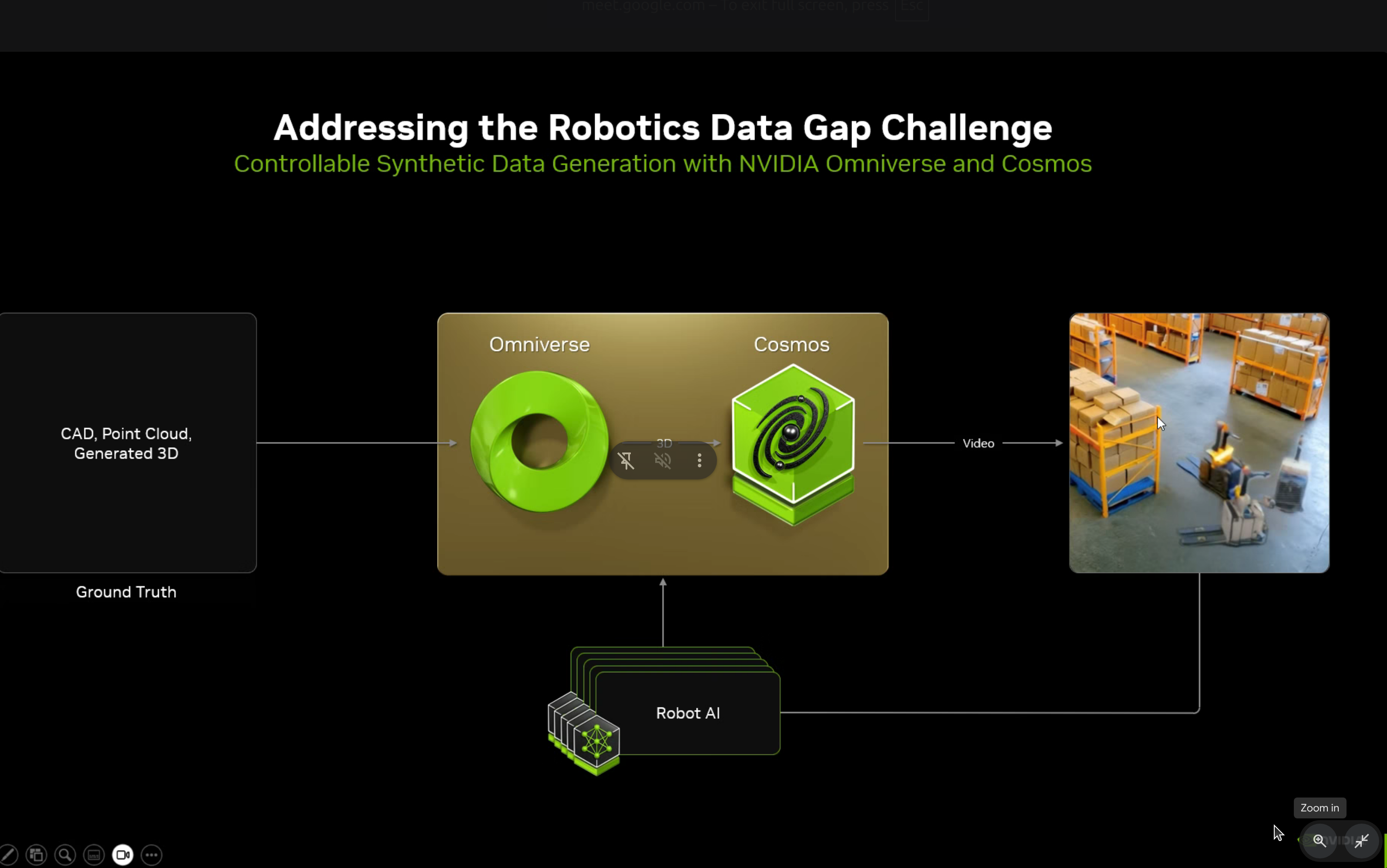
Cosmos Curator Data Pipeline
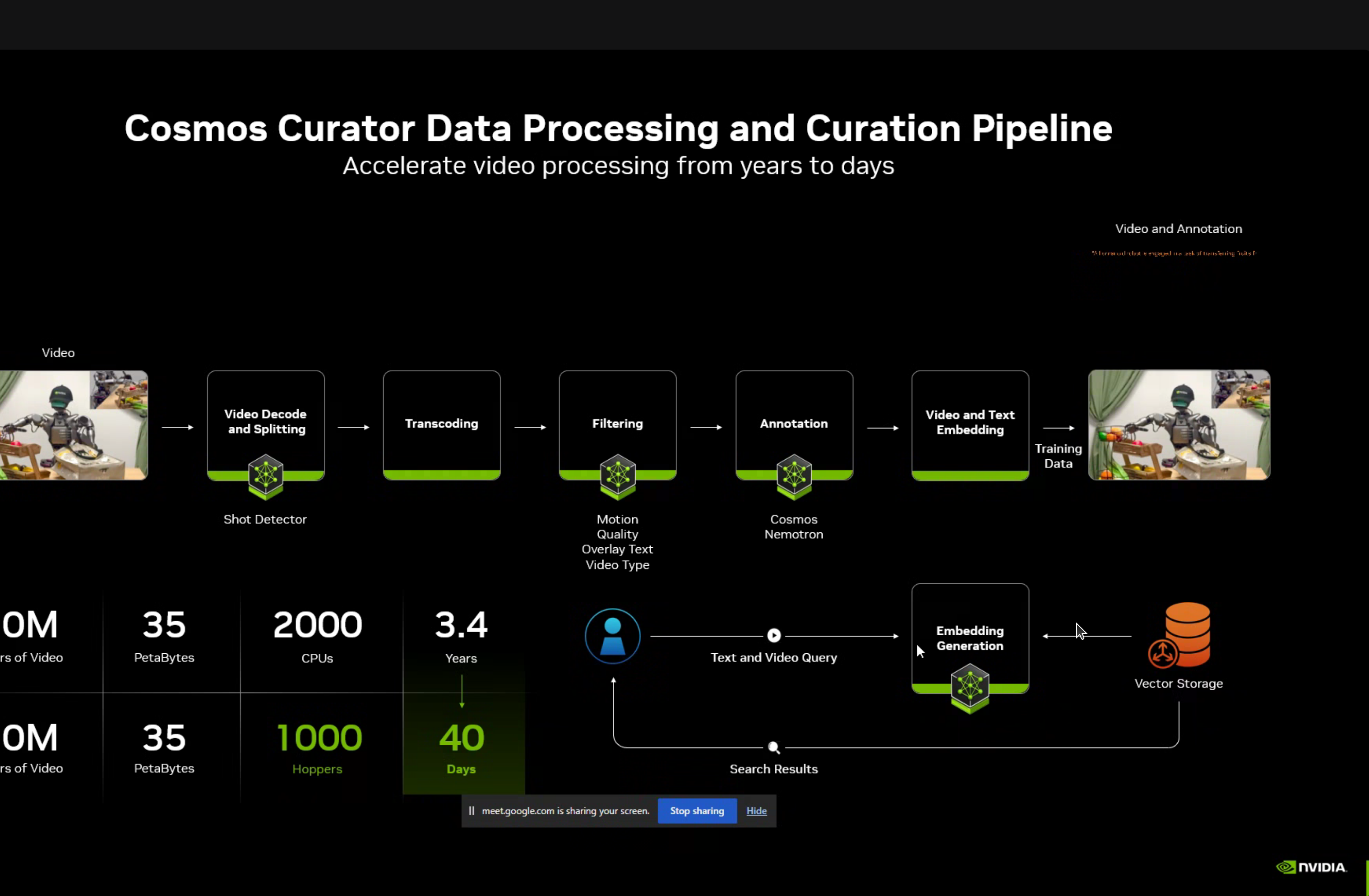
The Cosmos Curator provides accelerated data processing and curation, reducing processing time from 3.4 years to just 40 days for 20 million hours of video.
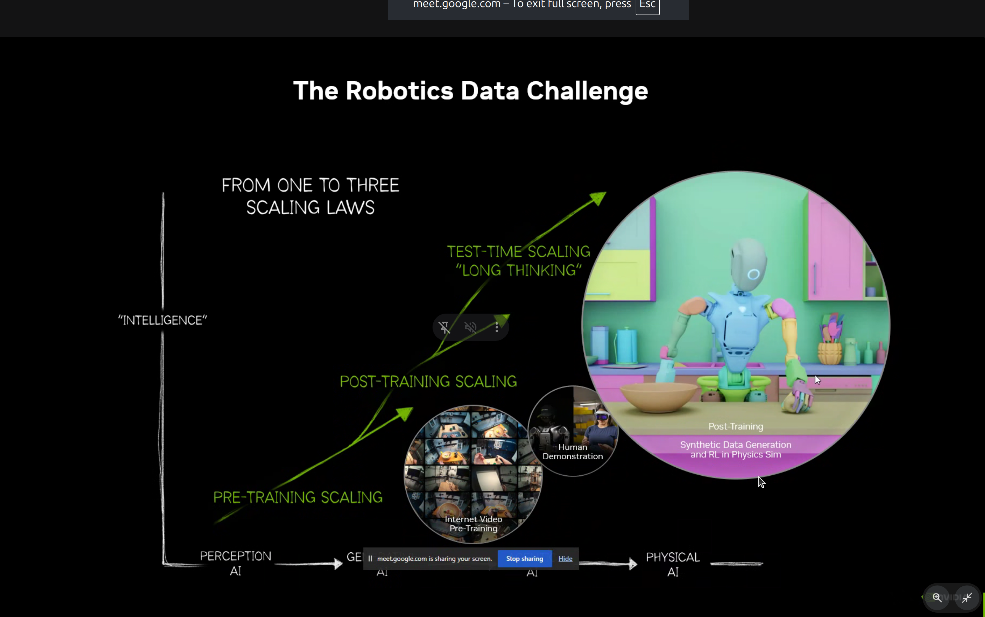
2. The Robotics Data Challenge
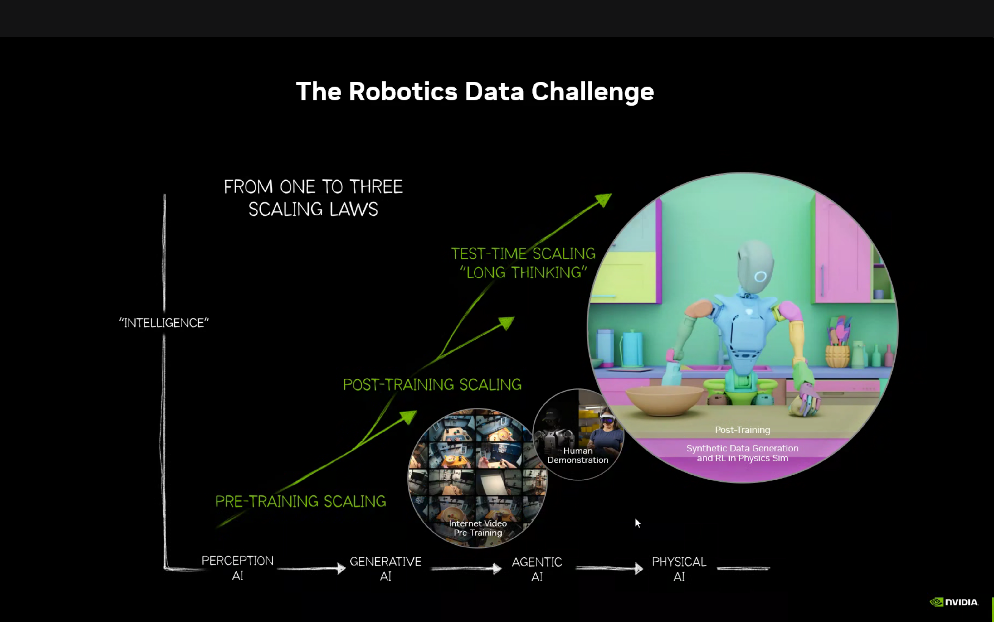
One of the key insights from the workshop was the evolution of scaling laws in AI:
Perception AI → Generative AI → Agentic AI → Physical AIPhysical AI requires three types of scaling:
- Pre-training Scaling - Internet video pre-training
- Post-training Scaling - Human demonstration + synthetic data generation
- Test-time Scaling - “Long thinking” for complex physical reasoning
3. Digital Twins & Synthetic Data
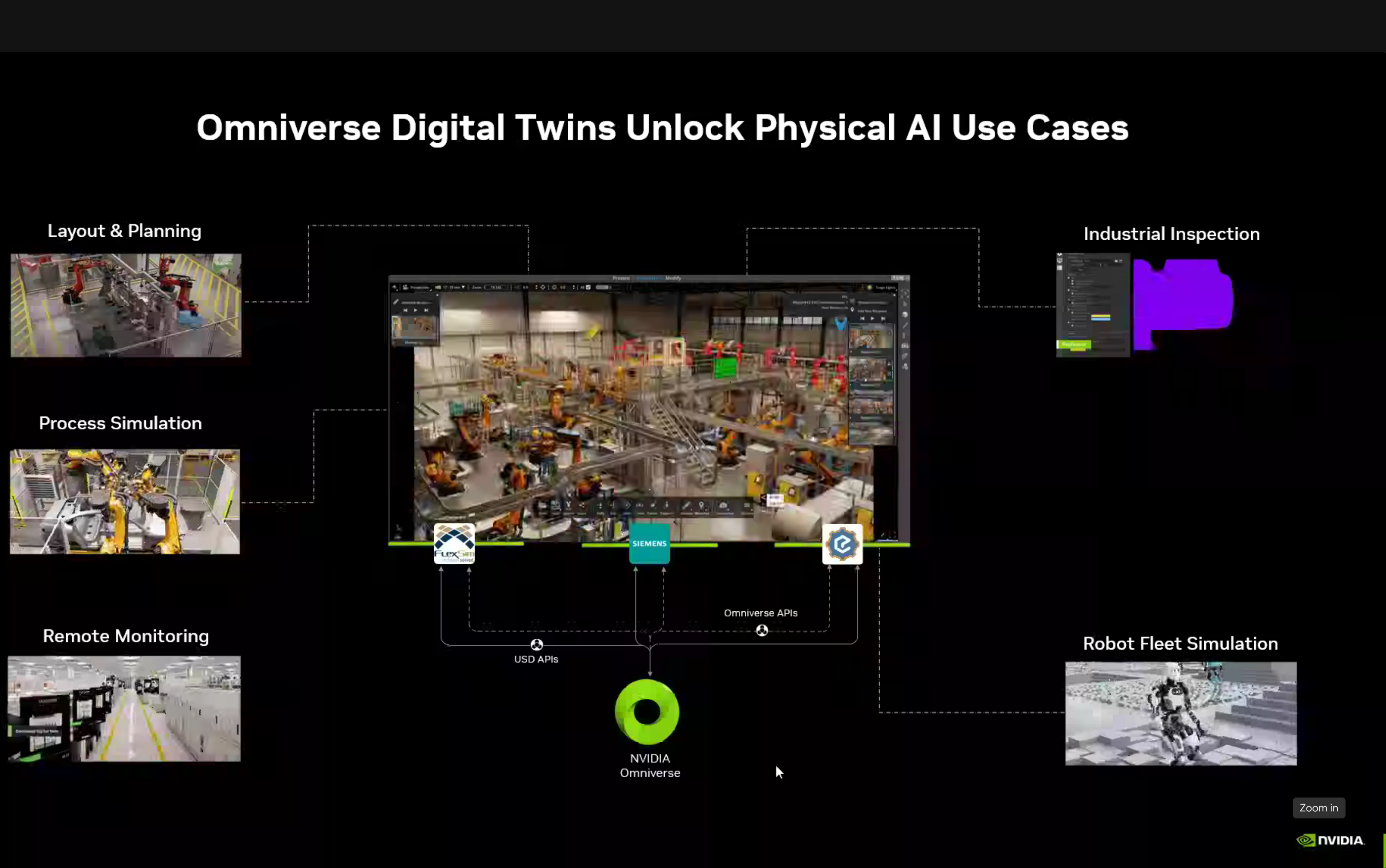
NVIDIA Omniverse Platform
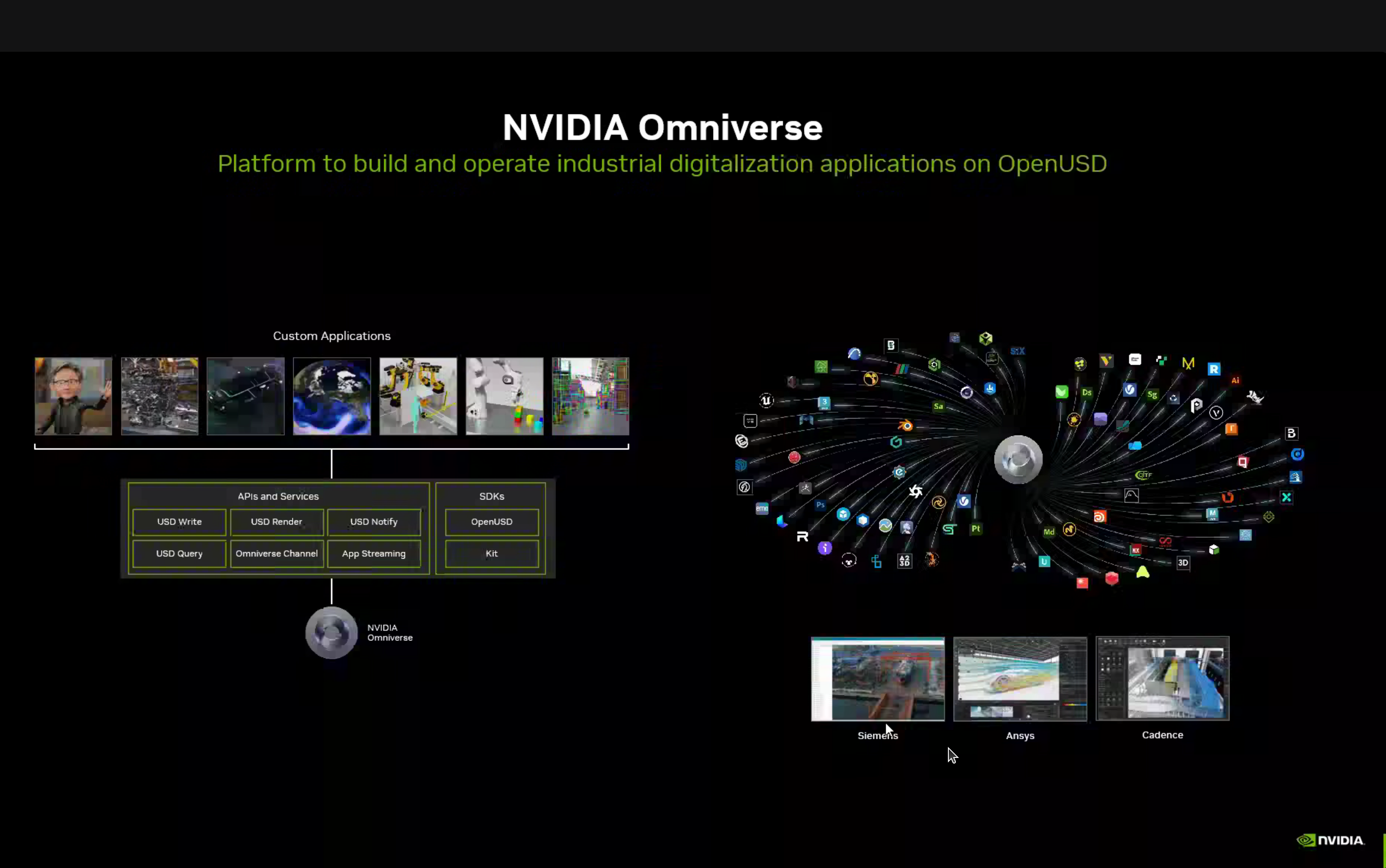
The Omniverse platform provides USD Write, USD Render, Omniverse Channel, App Streaming, SDKs, Operators, and Kit integration with various applications like Gazebo, Ansys, and Cadence.
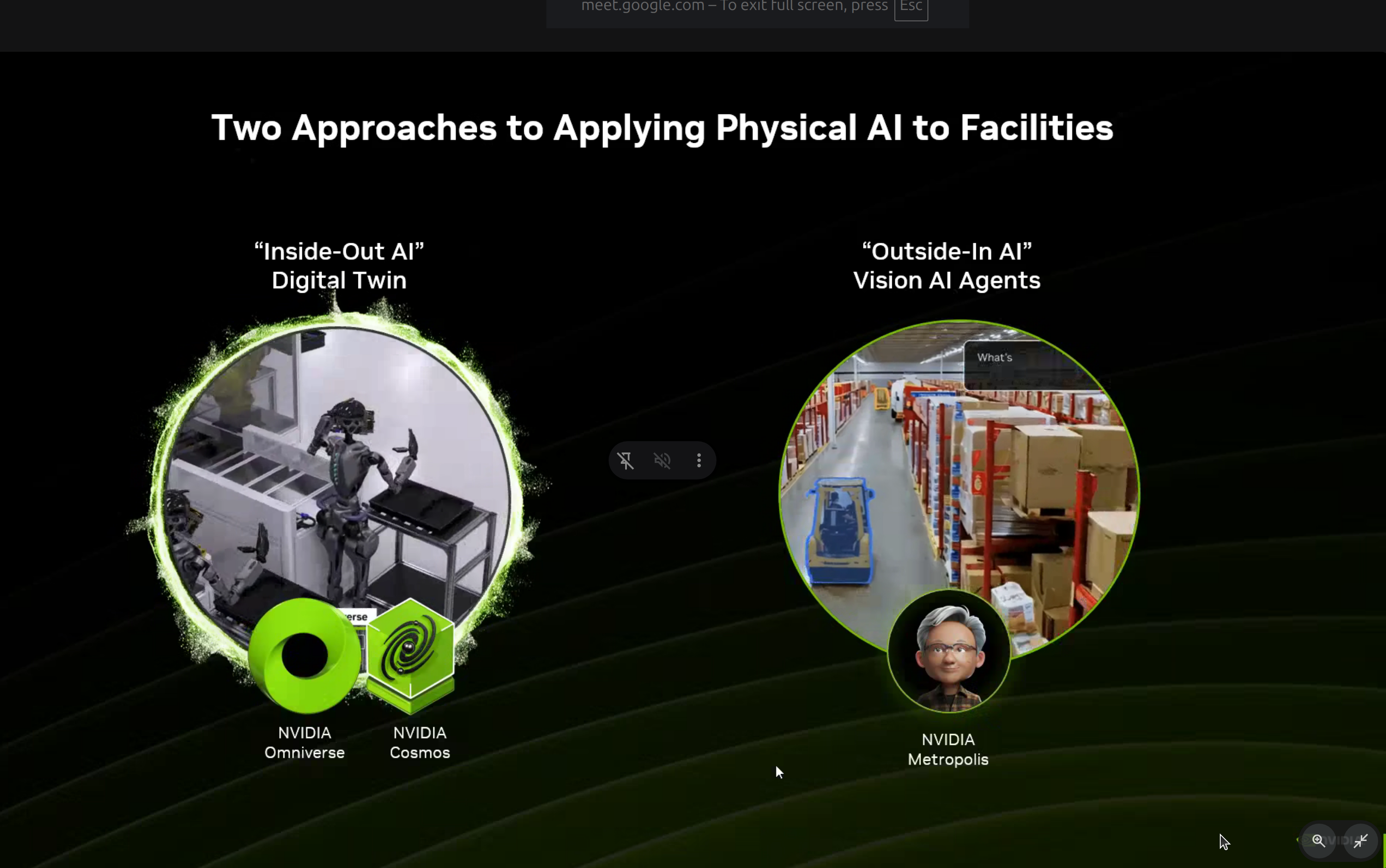
Two approaches to applying Physical AI:
- Inside-Out AI - Digital Twin using NVIDIA Omniverse and Cosmos
- Outside-In AI - Vision AI Agents using NVIDIA Metropolis
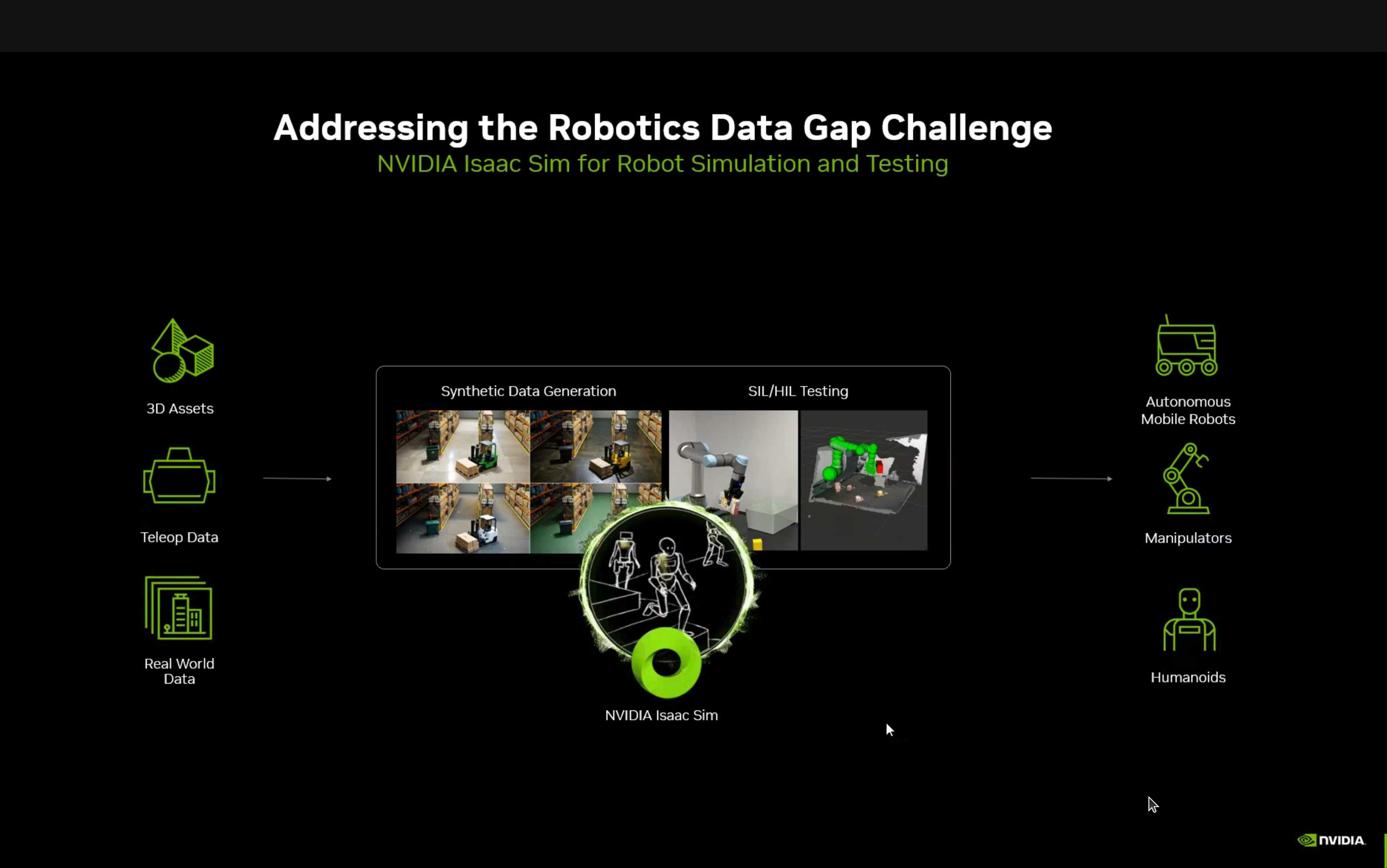
NVIDIA Isaac Platform
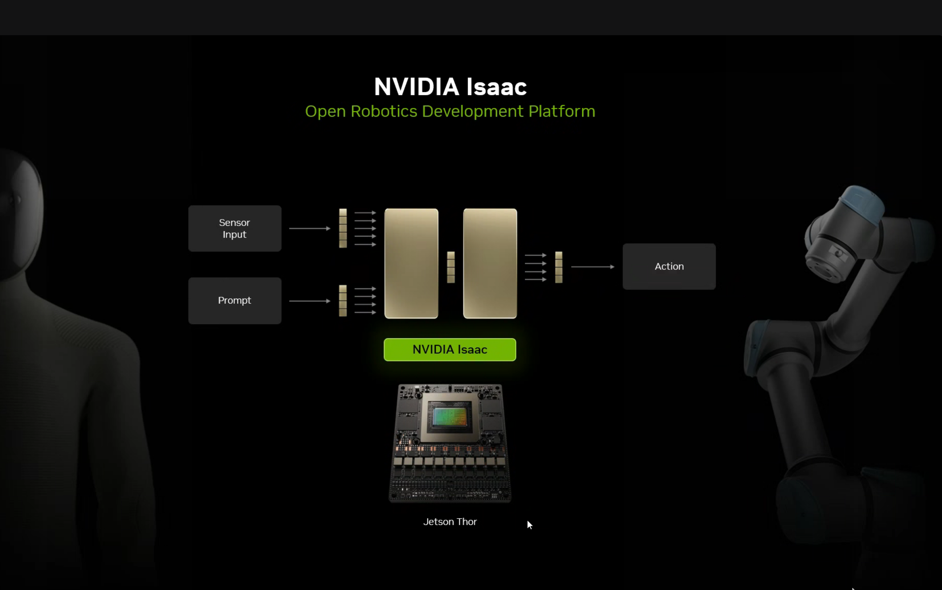
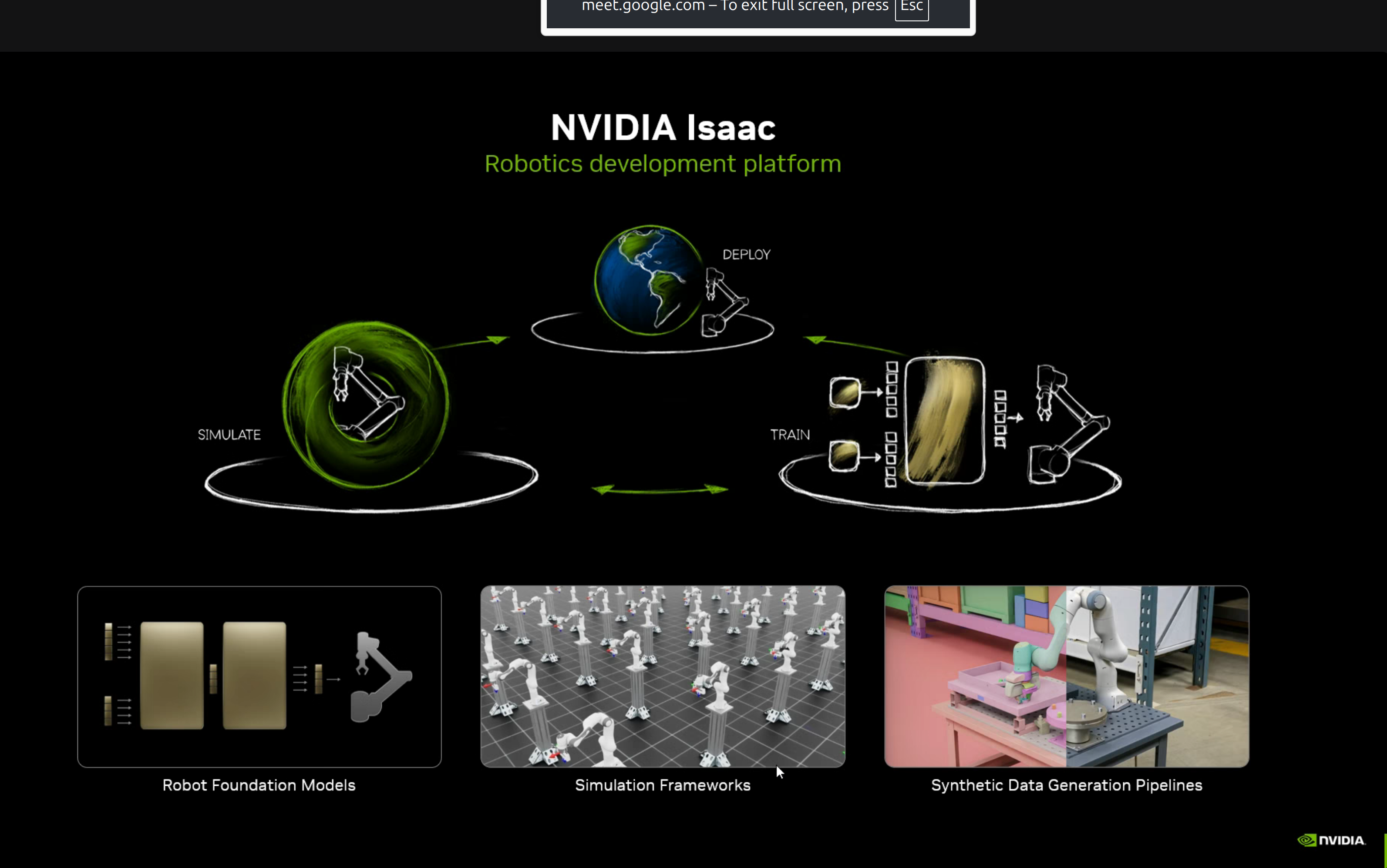
The NVIDIA Isaac platform provides:
- Robot Foundation Models - Pre-trained models for robotics tasks
- Simulation Frameworks - Physics simulation for training
- Synthetic Data Generation Pipelines - Data multiplication for training
Isaac Perceptor for Mobile Robots
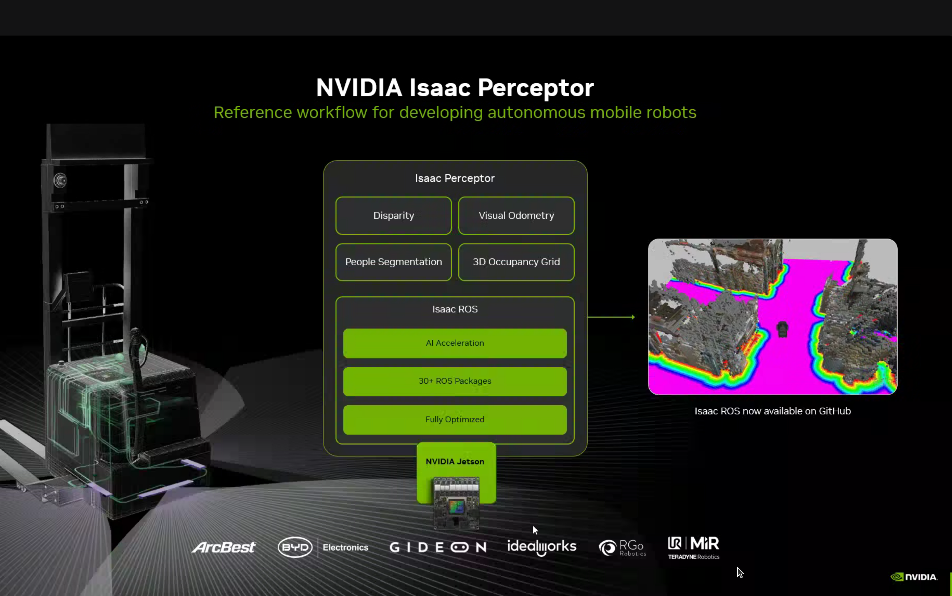
Isaac Perceptor is a reference workflow for developing autonomous mobile robots with:
- Disparity computation
- Visual Odometry
- People Segmentation
- 3D Occupancy Grid
All optimized to run on NVIDIA Jetson with Isaac ROS (30+ ROS packages, fully optimized).
Isaac Manipulator
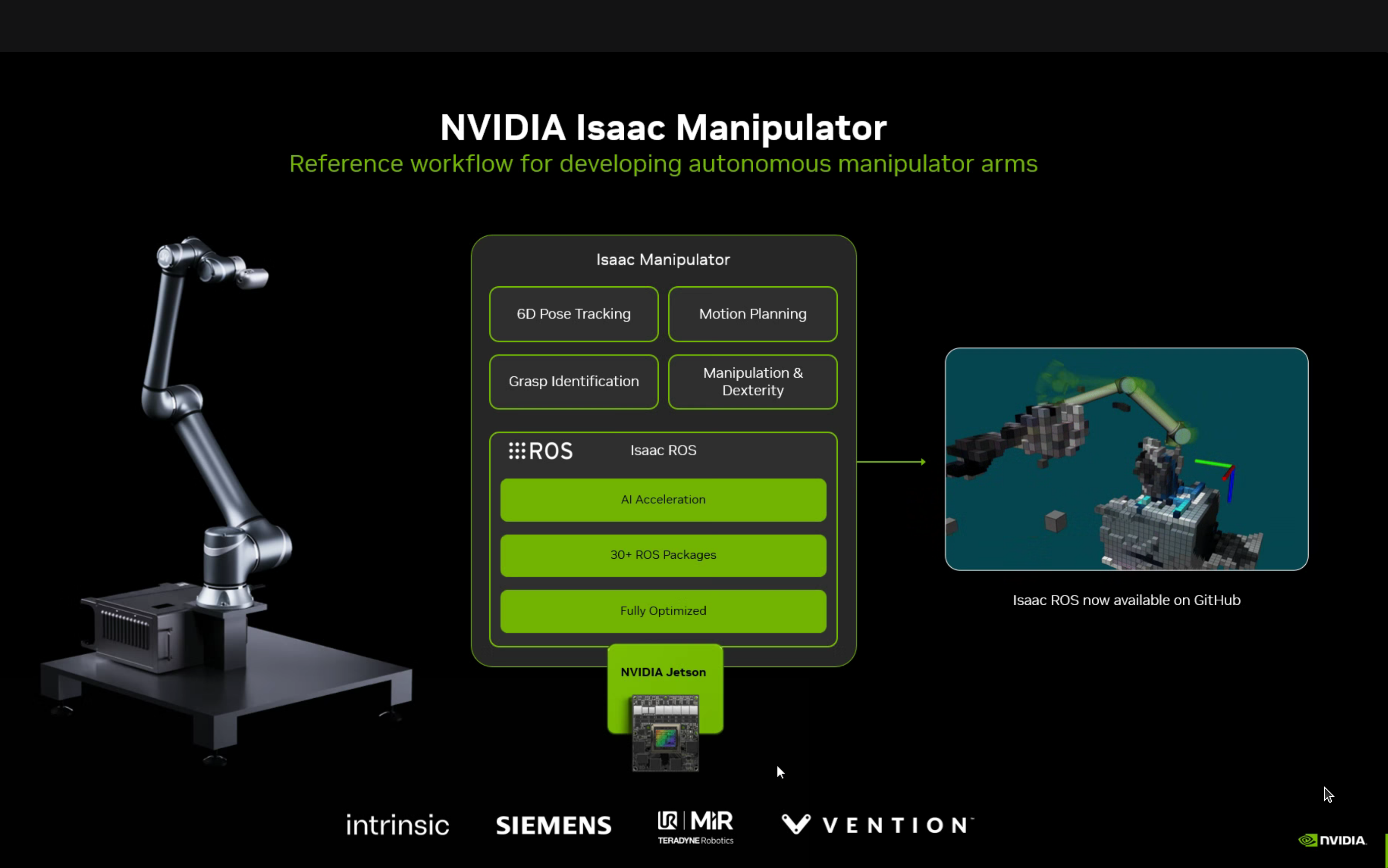
Reference workflow for robot arms with 6D Pose Tracking, Motion Planning, Grasp Identification, and Manipulation & Dexterity capabilities.
Isaac GROOT for Humanoids
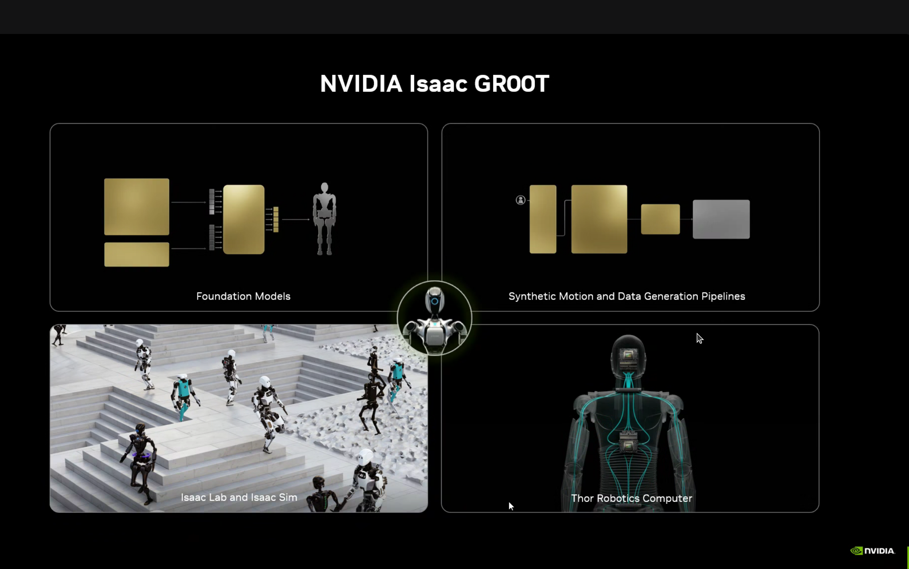
GROOT provides:
- Foundation Models - Pre-trained for humanoid robots
- Synthetic Motion and Data Generation Pipelines
- Isaac Lab and Isaac Sim - Simulation environment
- Thor Robotics Computer - Hardware platform
GROOT-Mimic Blueprint
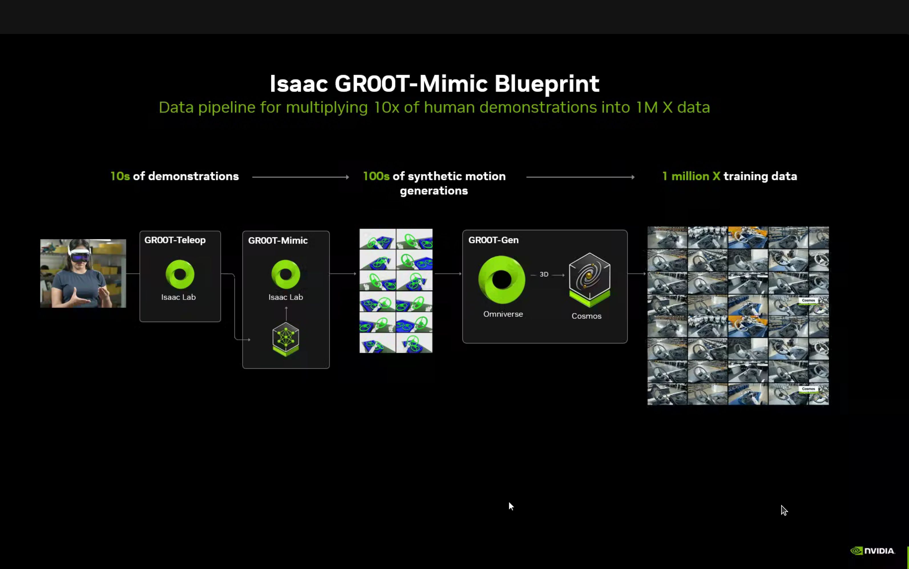
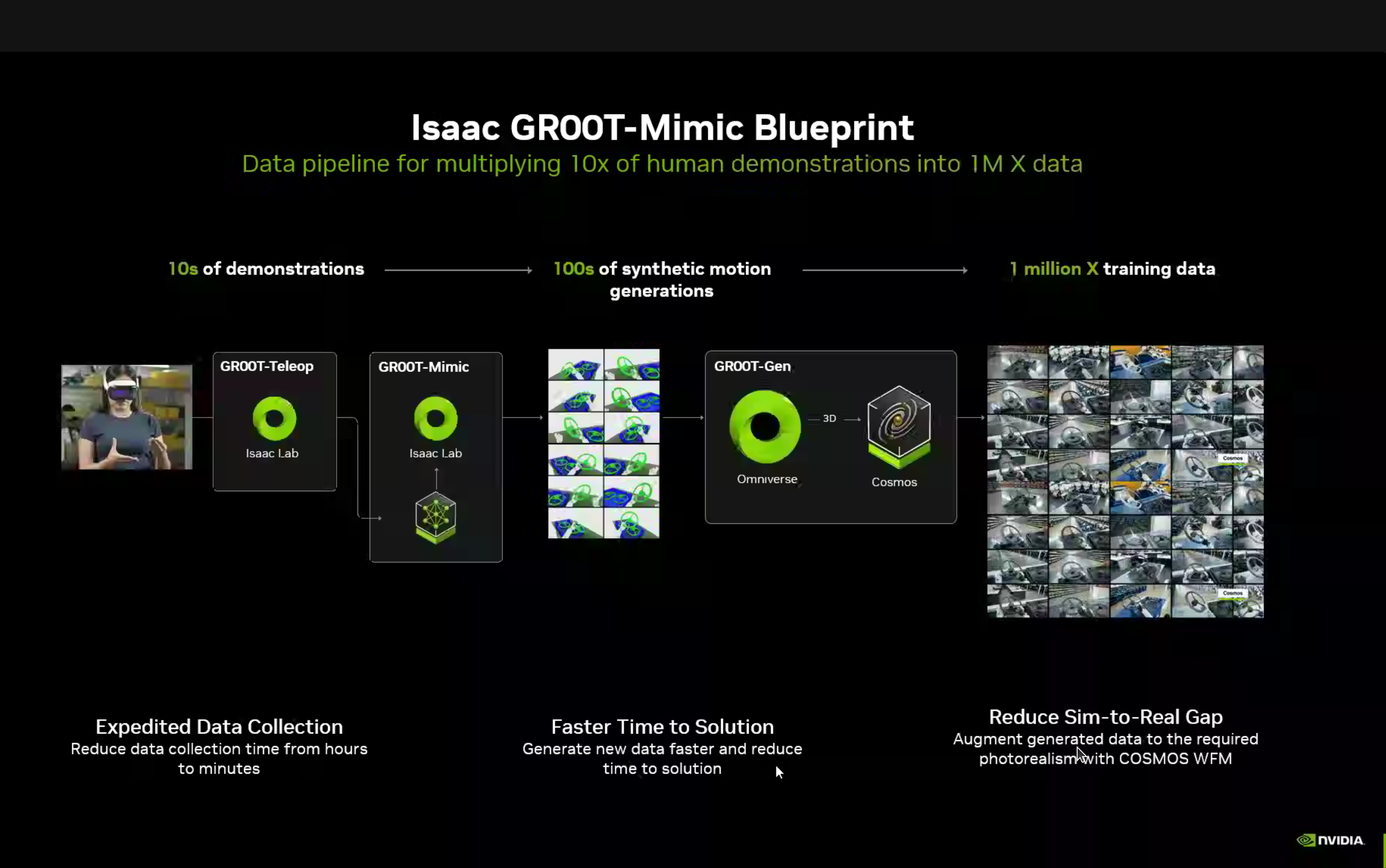
A fascinating data multiplication pipeline:
10s of demonstrations → 100s of synthetic motions → 1 Million training examplesThe pipeline components:
- GROOT-Teleop (Isaac Lab) - Capture human demonstrations via teleoperation
- GROOT-Mimic (Isaac Lab) - Learn motion patterns from demonstrations
- GROOT-Gen (Omniverse + Cosmos) - Generate synthetic variations at scale
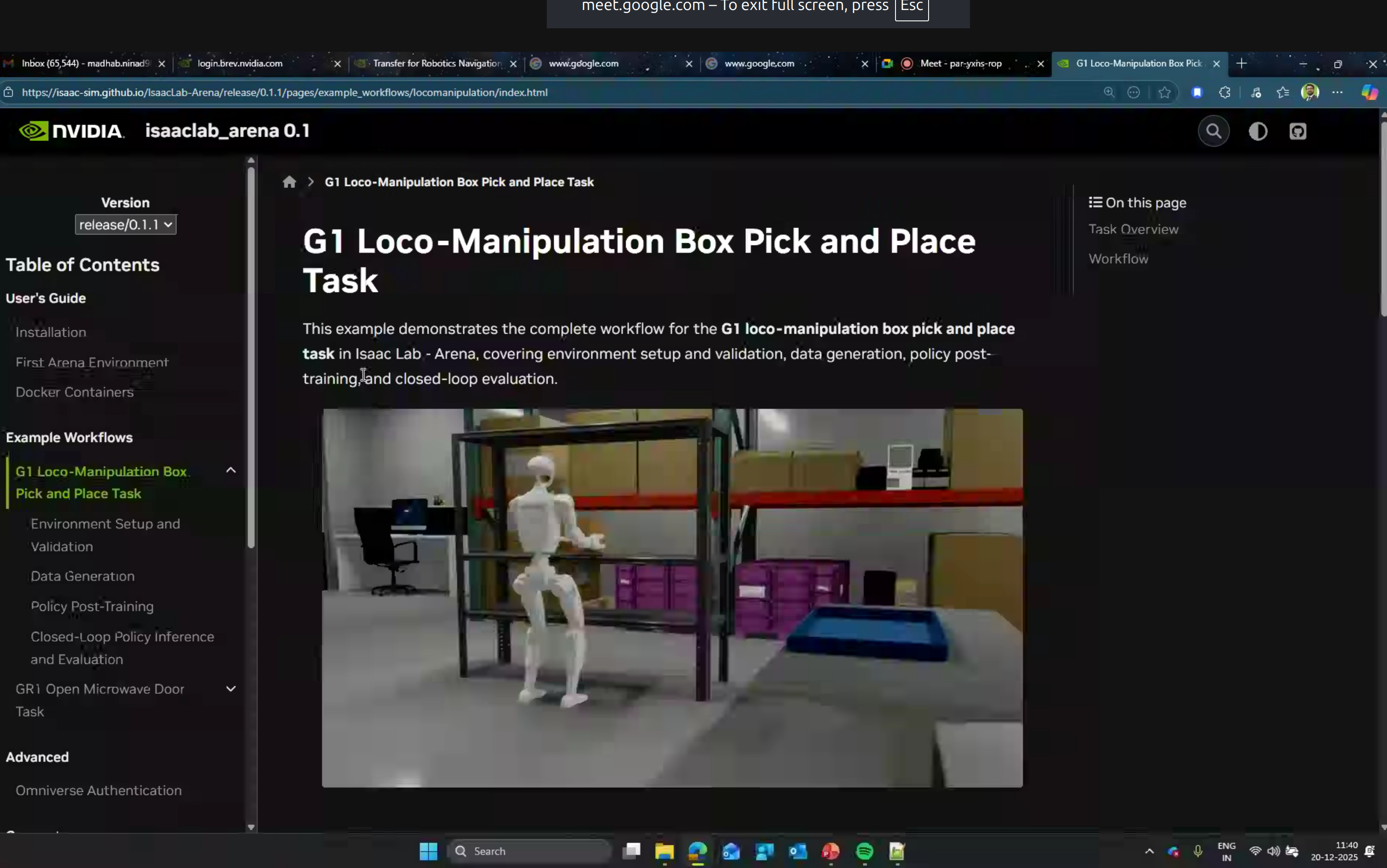
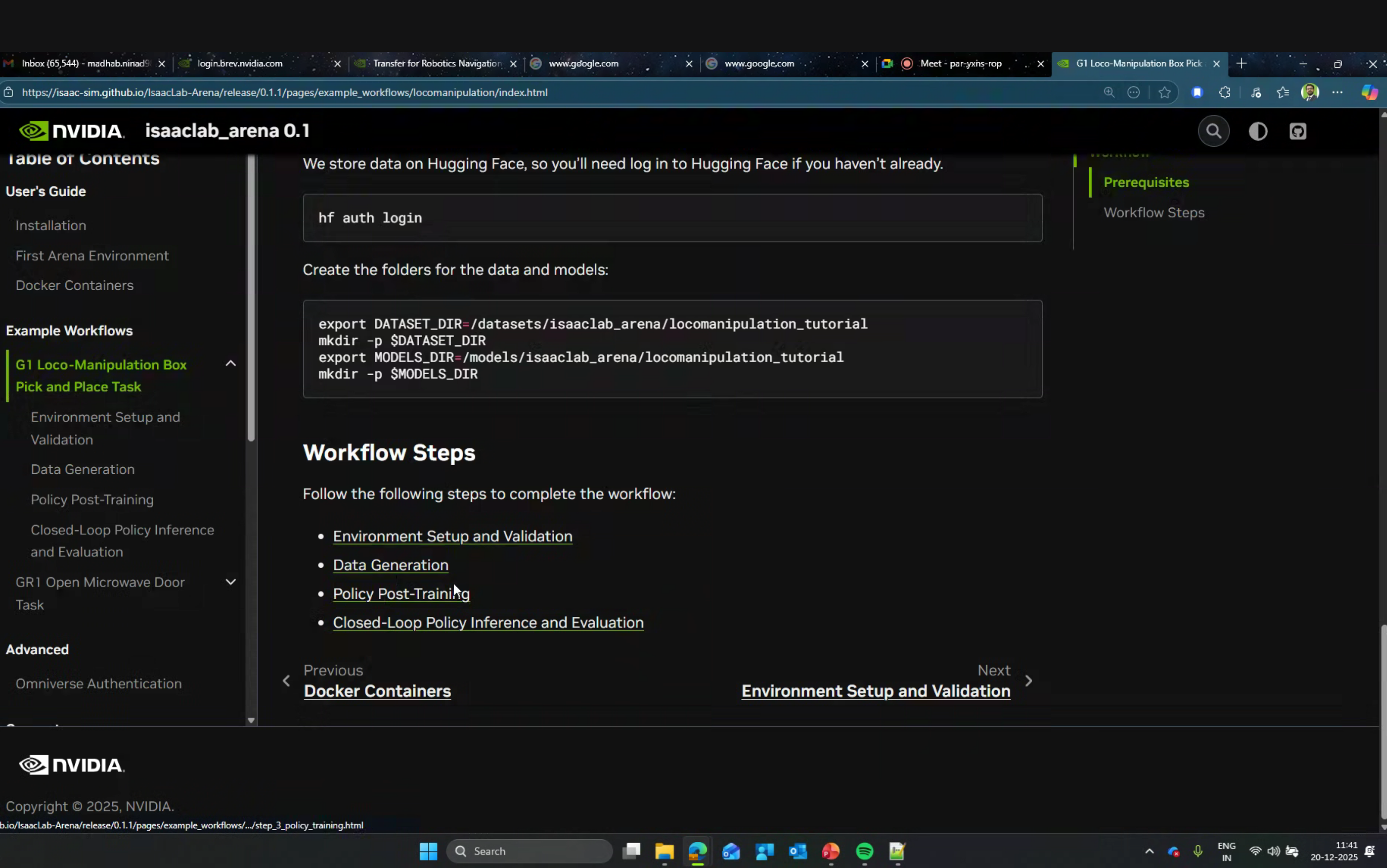
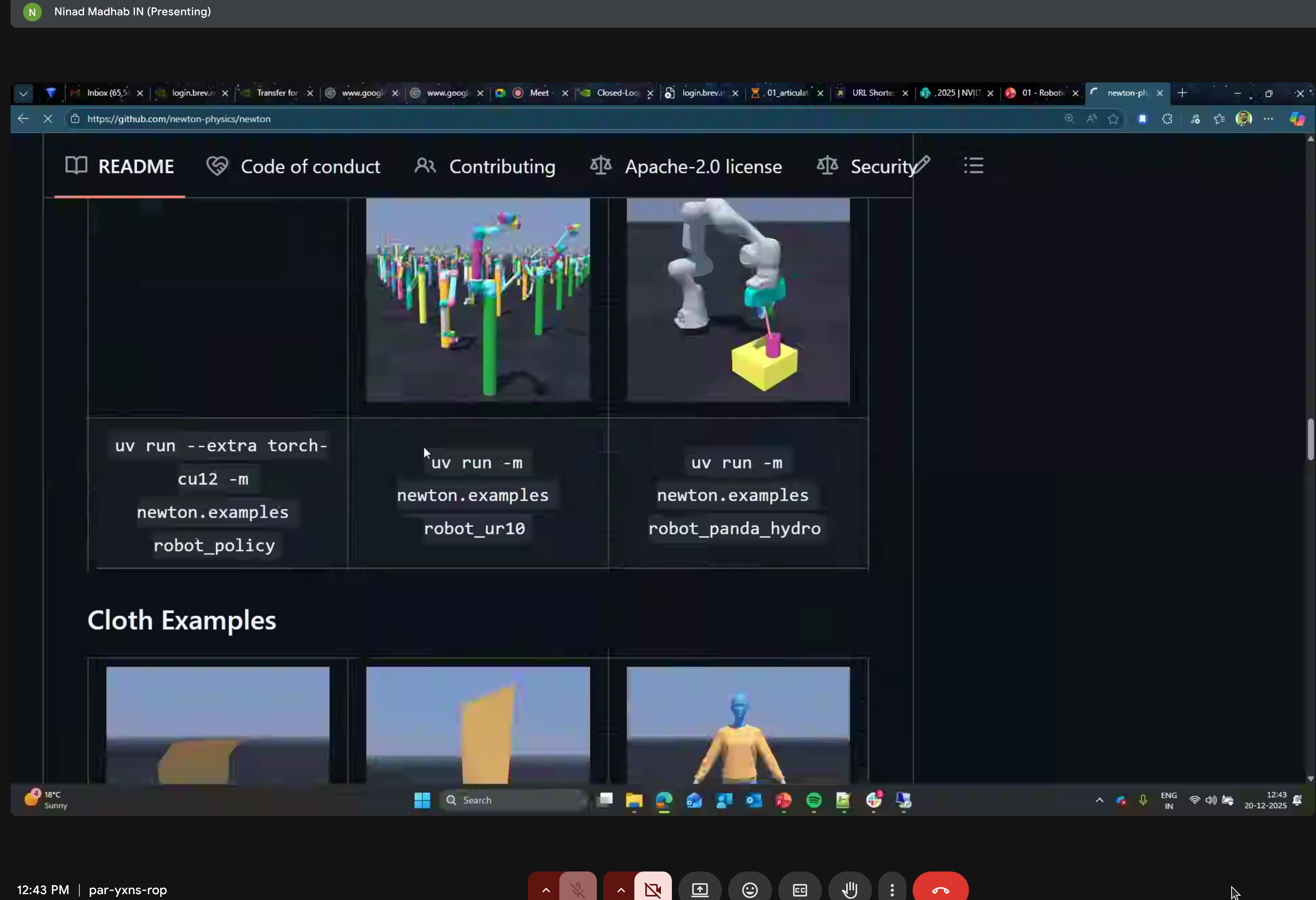
Isaac Lab Arena Tutorials
Newton Physics Engine
The main focus of the hands-on portion was Newton - NVIDIA’s new physics simulation engine.
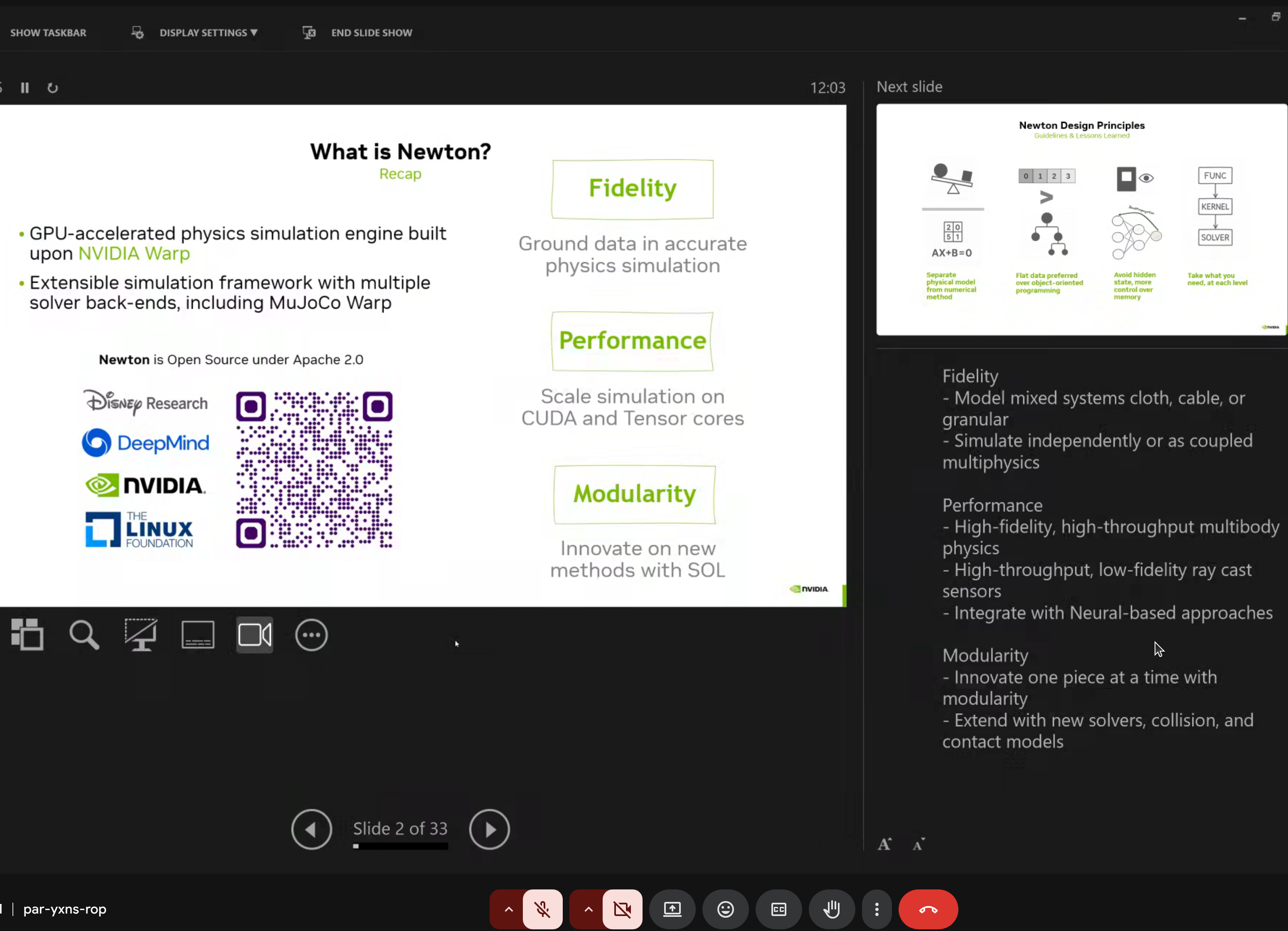
What is Newton?

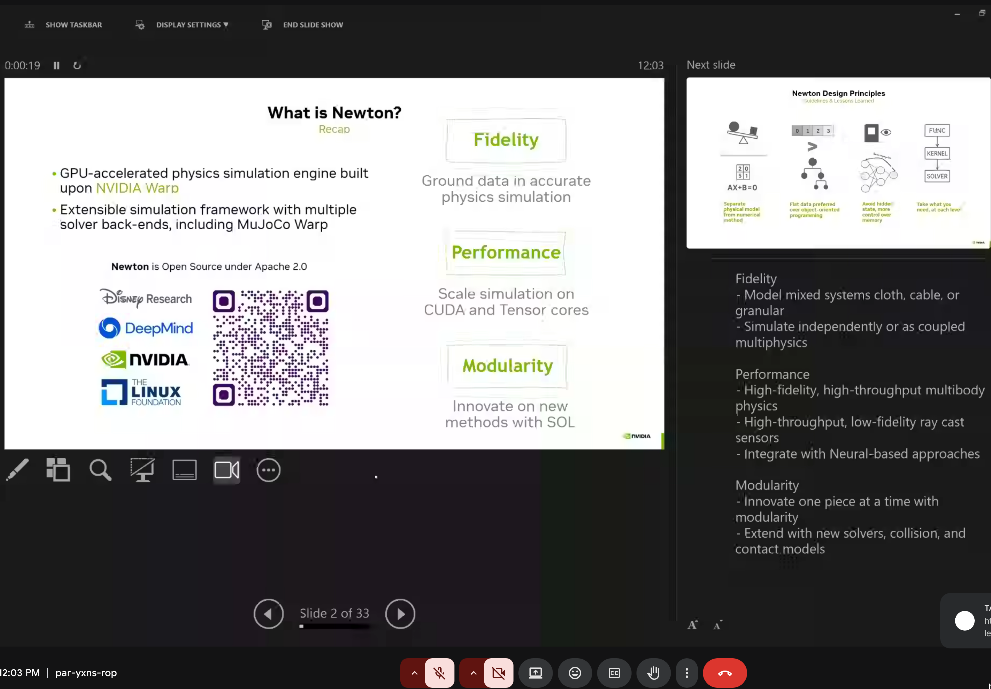
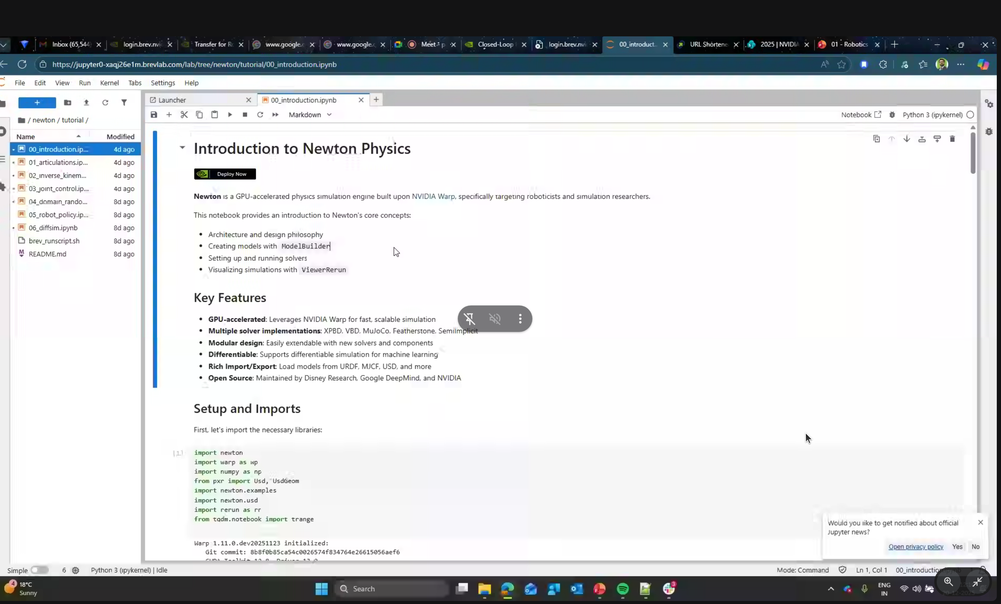
Newton is a GPU-accelerated physics simulation engine built upon NVIDIA Warp, specifically targeting roboticists and simulation researchers.
Key Characteristics:
- Open Source - Apache 2.0 license
- GPU-Accelerated - Leverages NVIDIA Warp for fast, scalable simulation
- Differentiable - Supports gradient computation for machine learning
- Modular - Easily extensible with new solvers and components
Backed by Industry Leaders:
- Disney Research
- Google DeepMind
- NVIDIA
- The Linux Foundation
Newton Design Principles
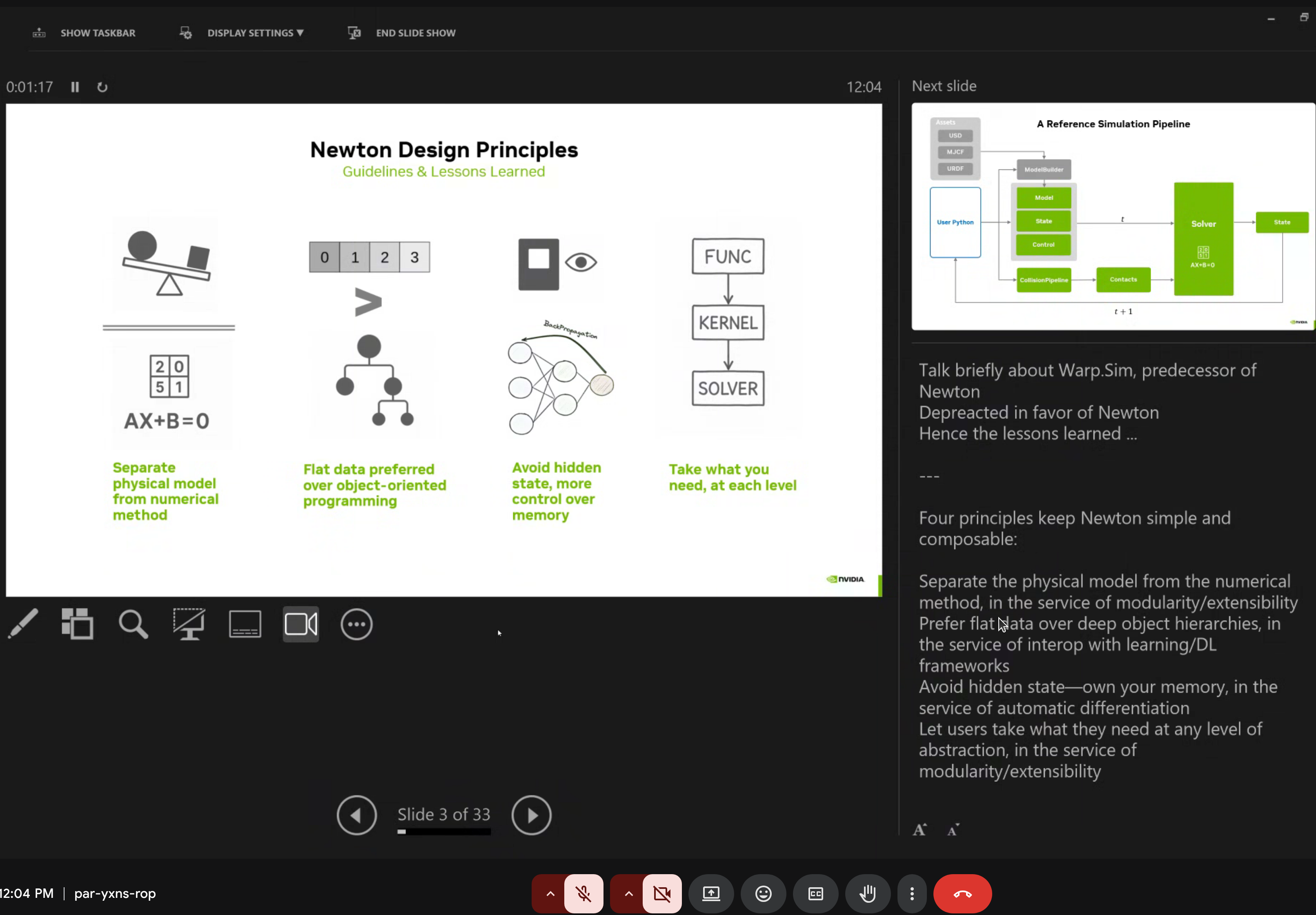
Newton follows four core design guidelines:
- Separate physical model from numerical method (AX+B=0)
- Flat data preferred over object-oriented programming
- Avoid hidden state for memory control
- Take what you need at each level (FUNC/KERNEL/SOLVER abstraction)
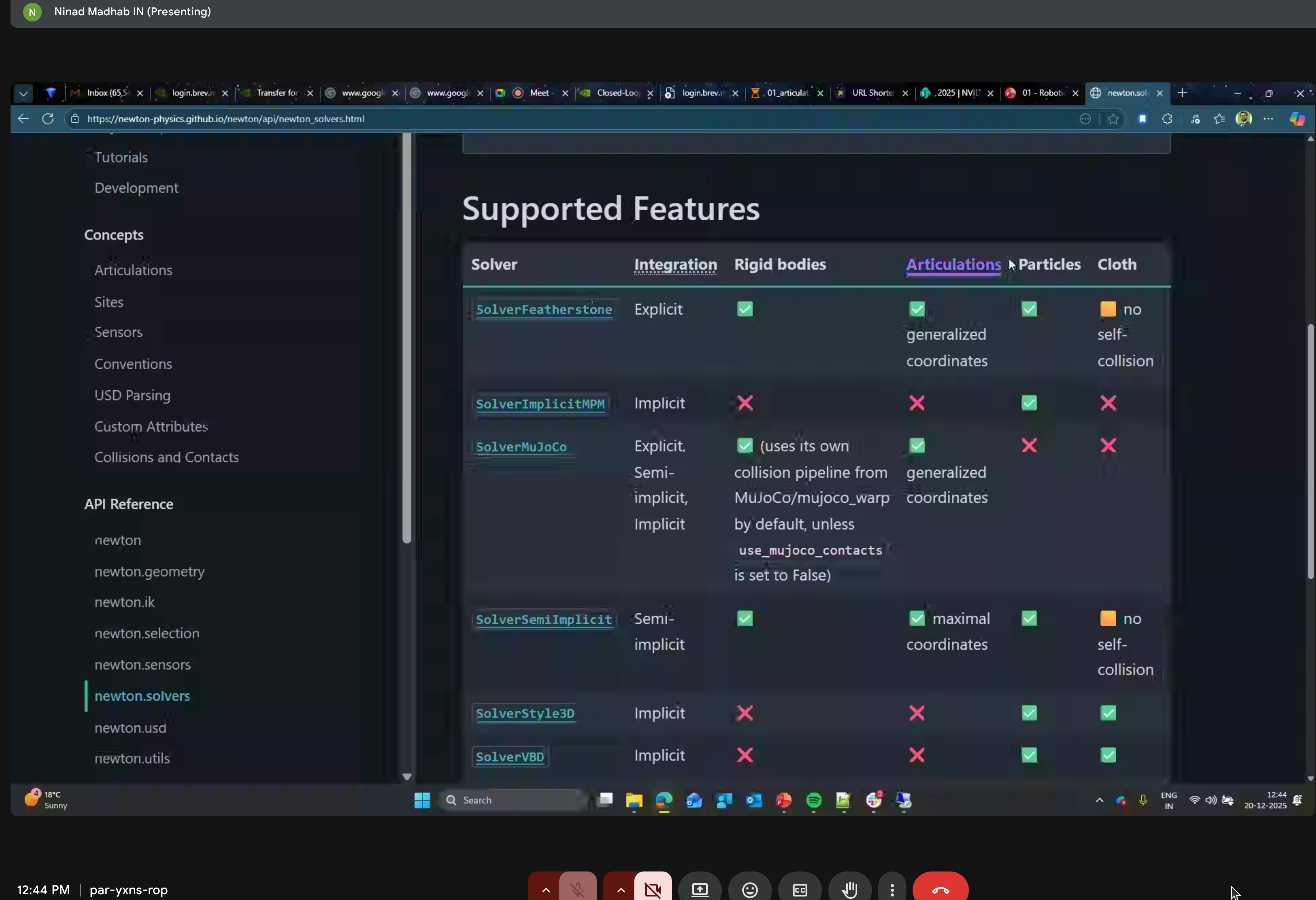
Core Features
| Feature | Description |
|---|---|
| Multiple Solvers | XPBD, VBD, MuJoCo, Featherstone, SemiImplicit |
| Rich Import/Export | URDF, MJCF, USD file formats |
| Modular Design | Easy to extend with custom solvers |
| Differentiable | End-to-end gradient support for RL |
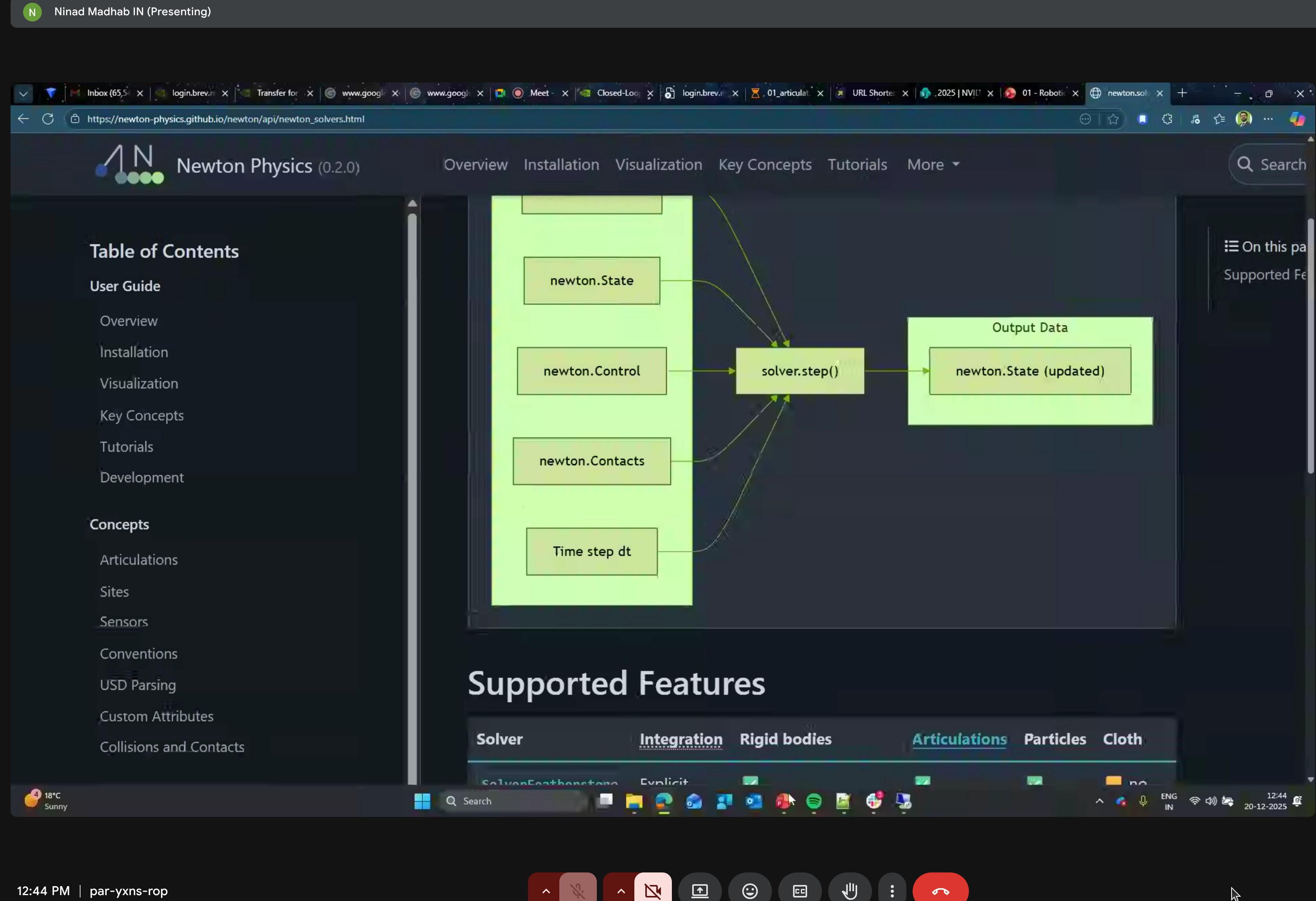
Newton Architecture
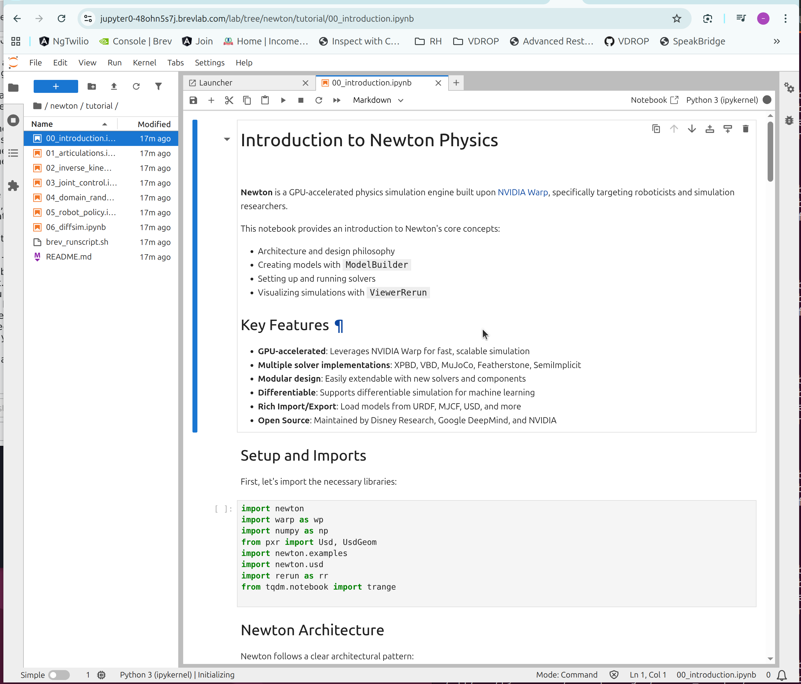
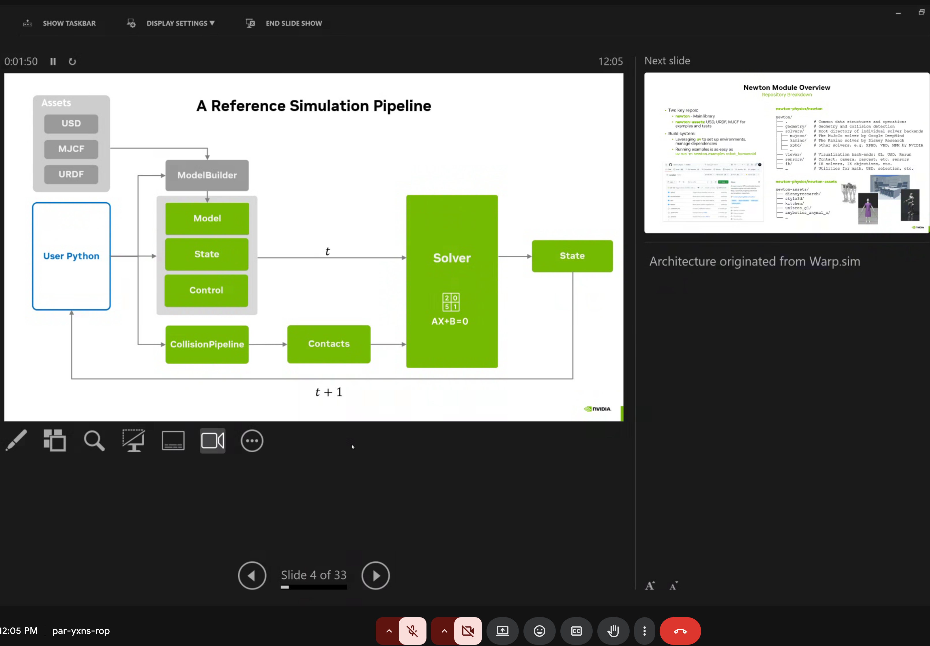
Newton follows a clean architectural pattern:
import newton
import warp as wp
import numpy as np
from pxr import Usd, UsdGeom
# Key modules
import newton.examples
import newton.usd
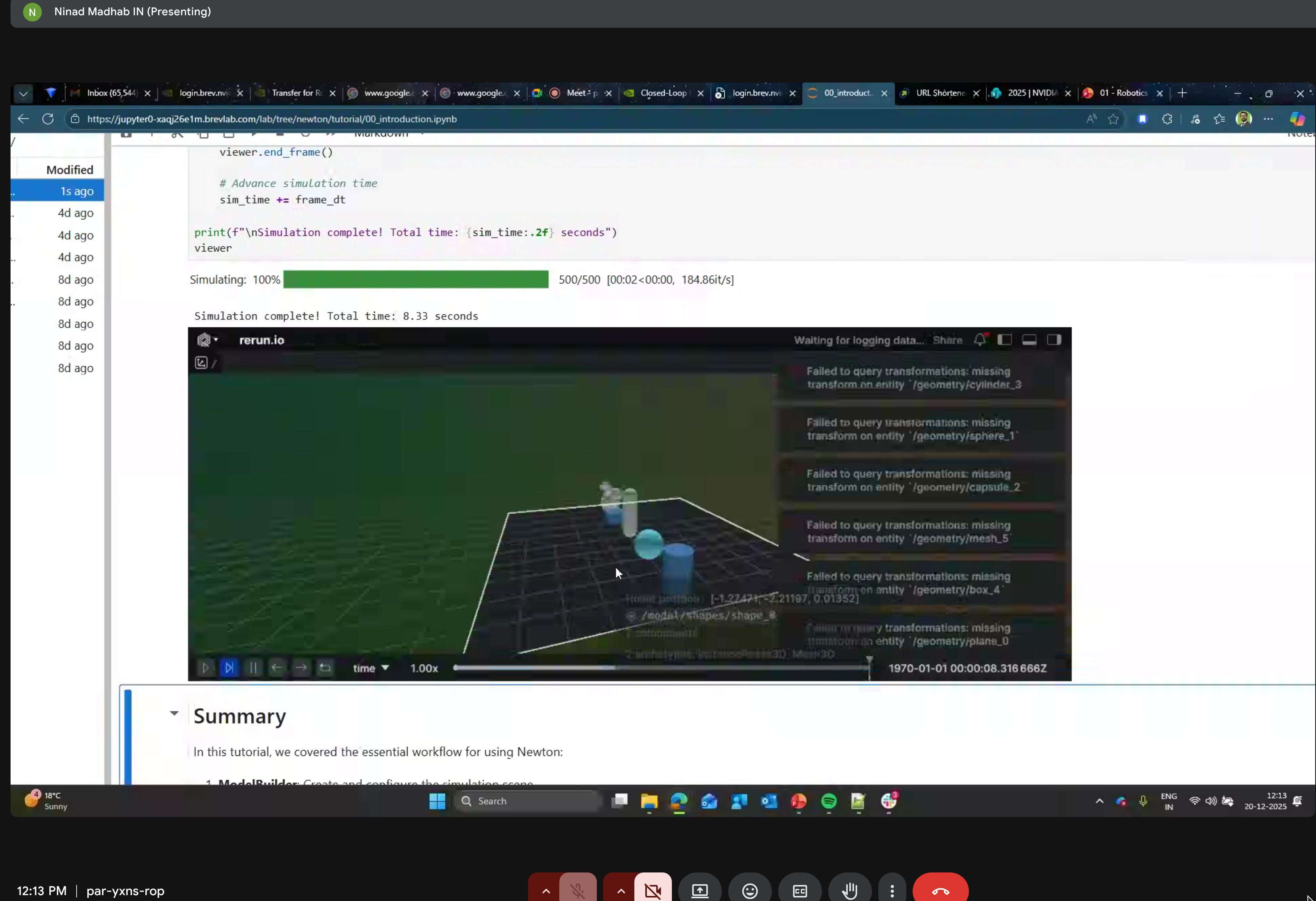
import rerun as rr # Visualization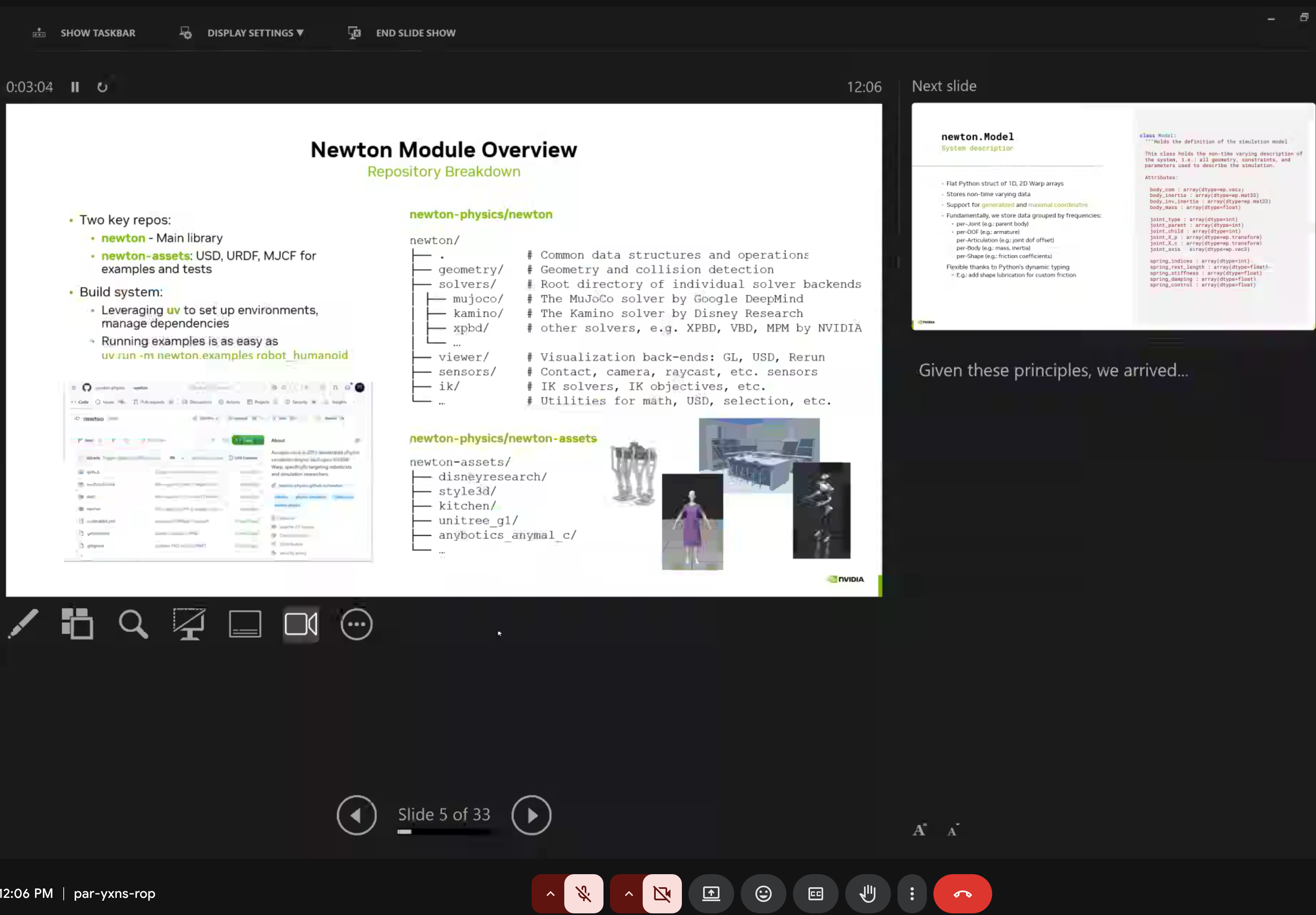
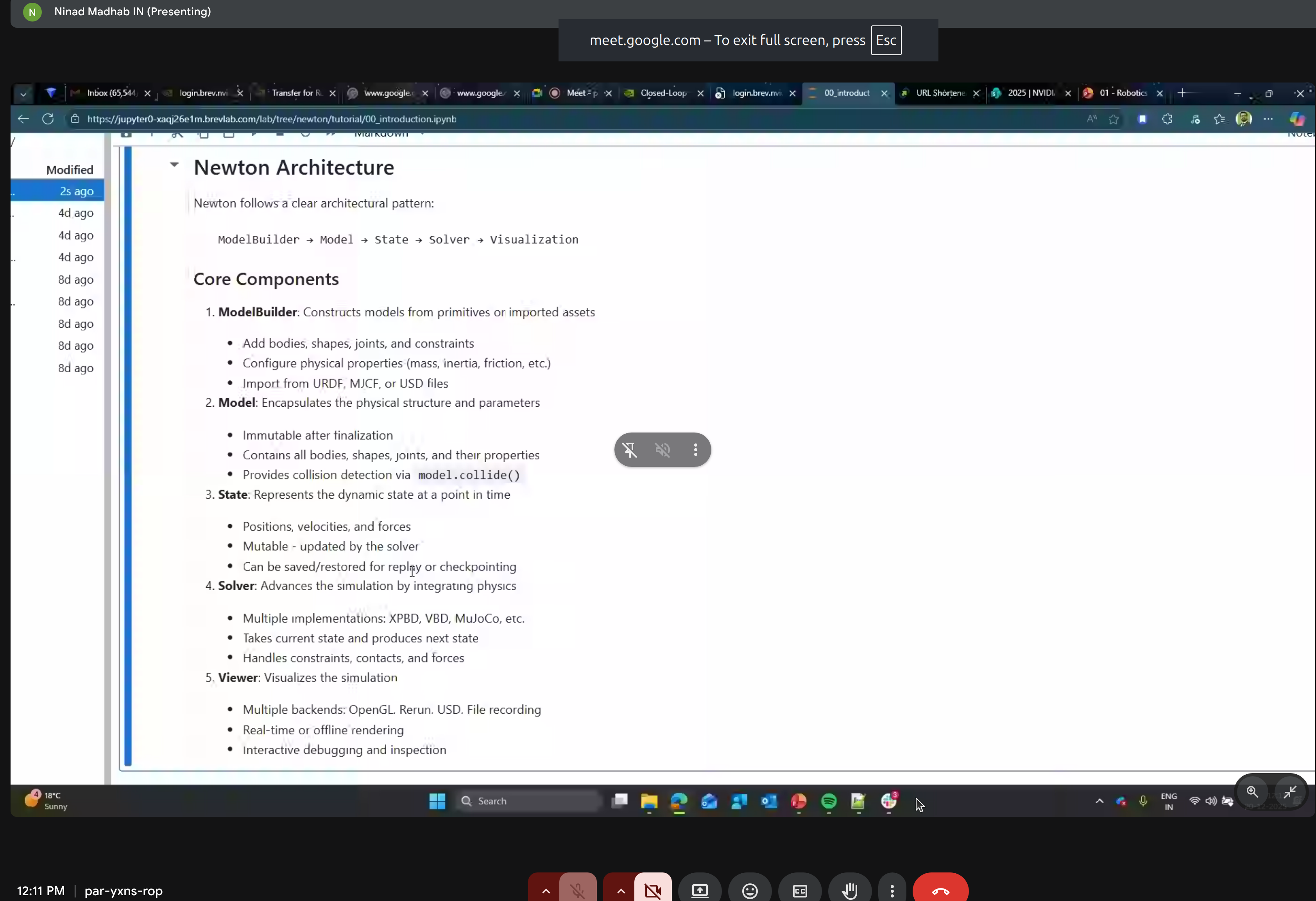
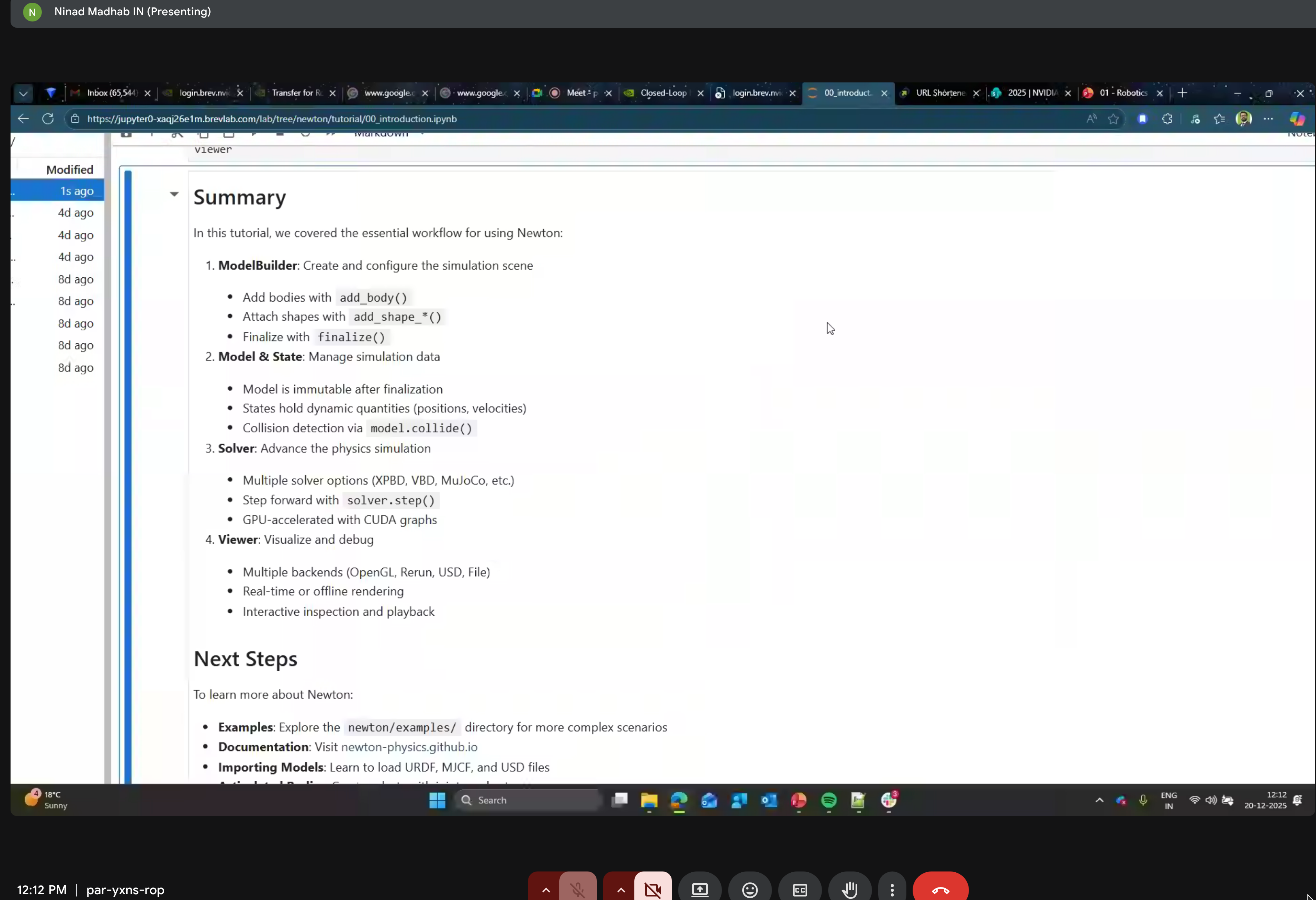
The five core components:
- ModelBuilder - Constructing models
- Model - Encapsulating physical structure
- State - Dynamic state representation
- Solver - Physics simulation
- Viewer - Visualization
Key Concepts
1. ModelBuilder
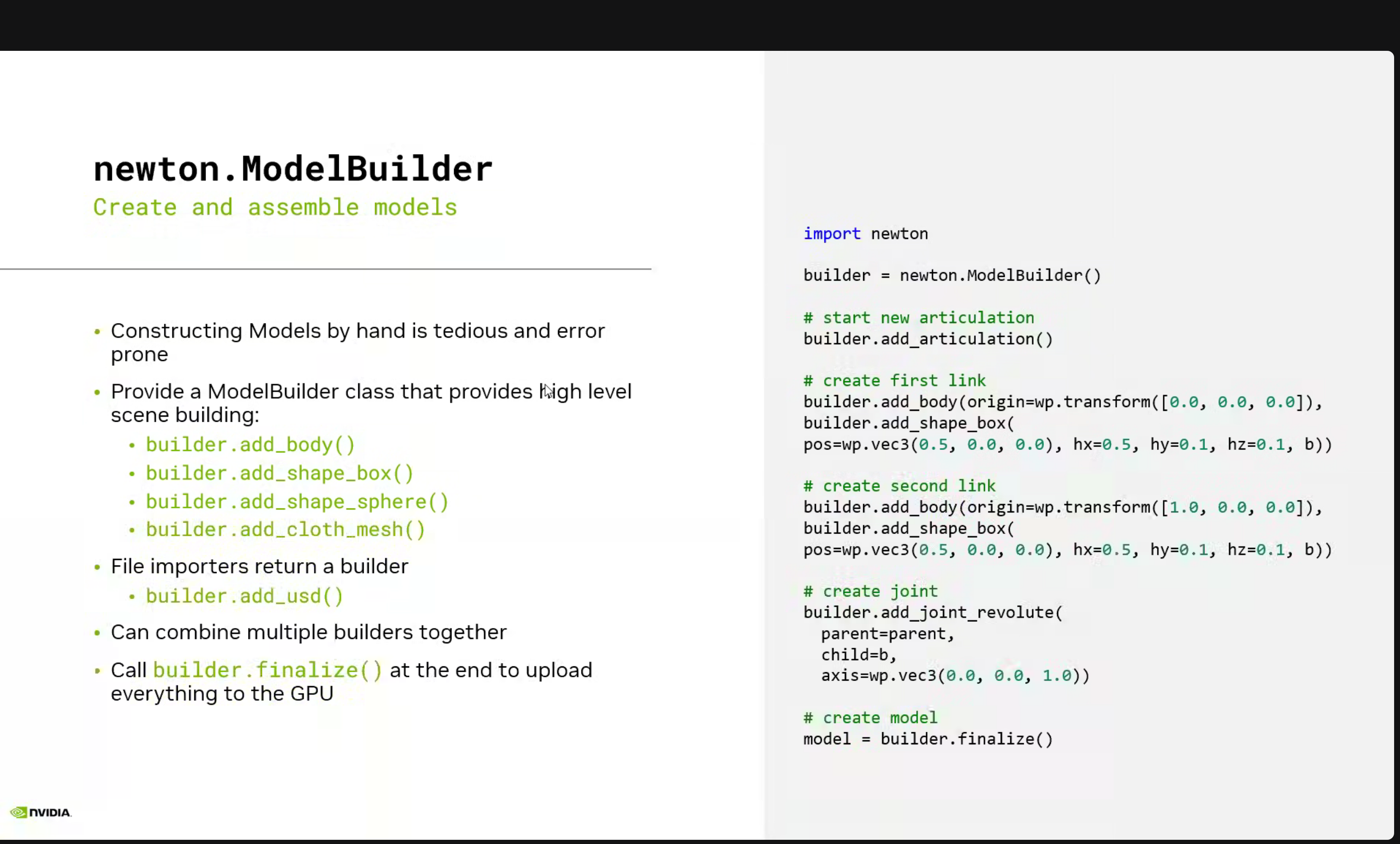
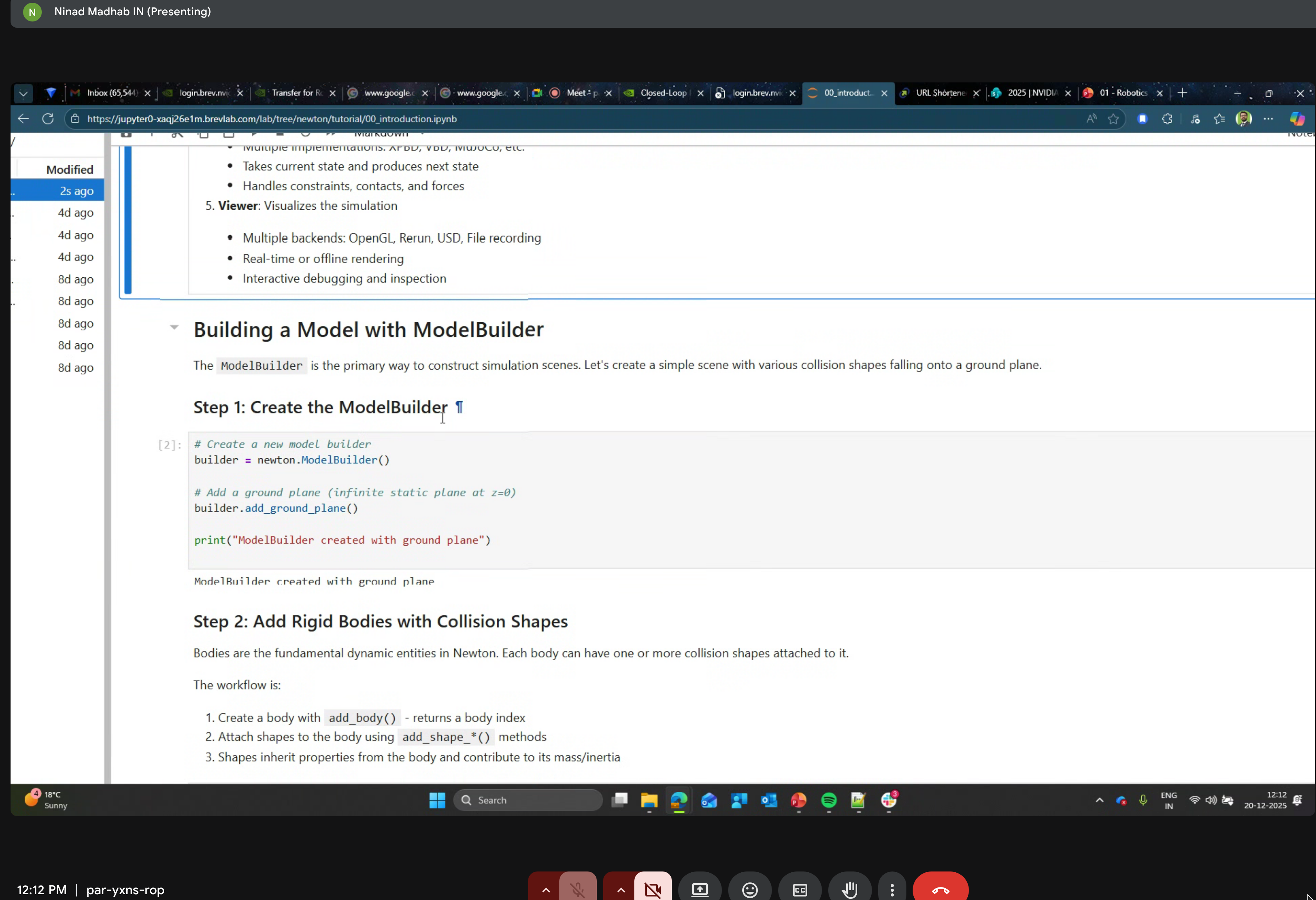
Create articulated systems programmatically or import from standard formats:
builder = newton.ModelBuilder()
builder.add_usd("cartpole.usd")

# Finalize and upload to GPU
model = builder.finalize()
2. Model
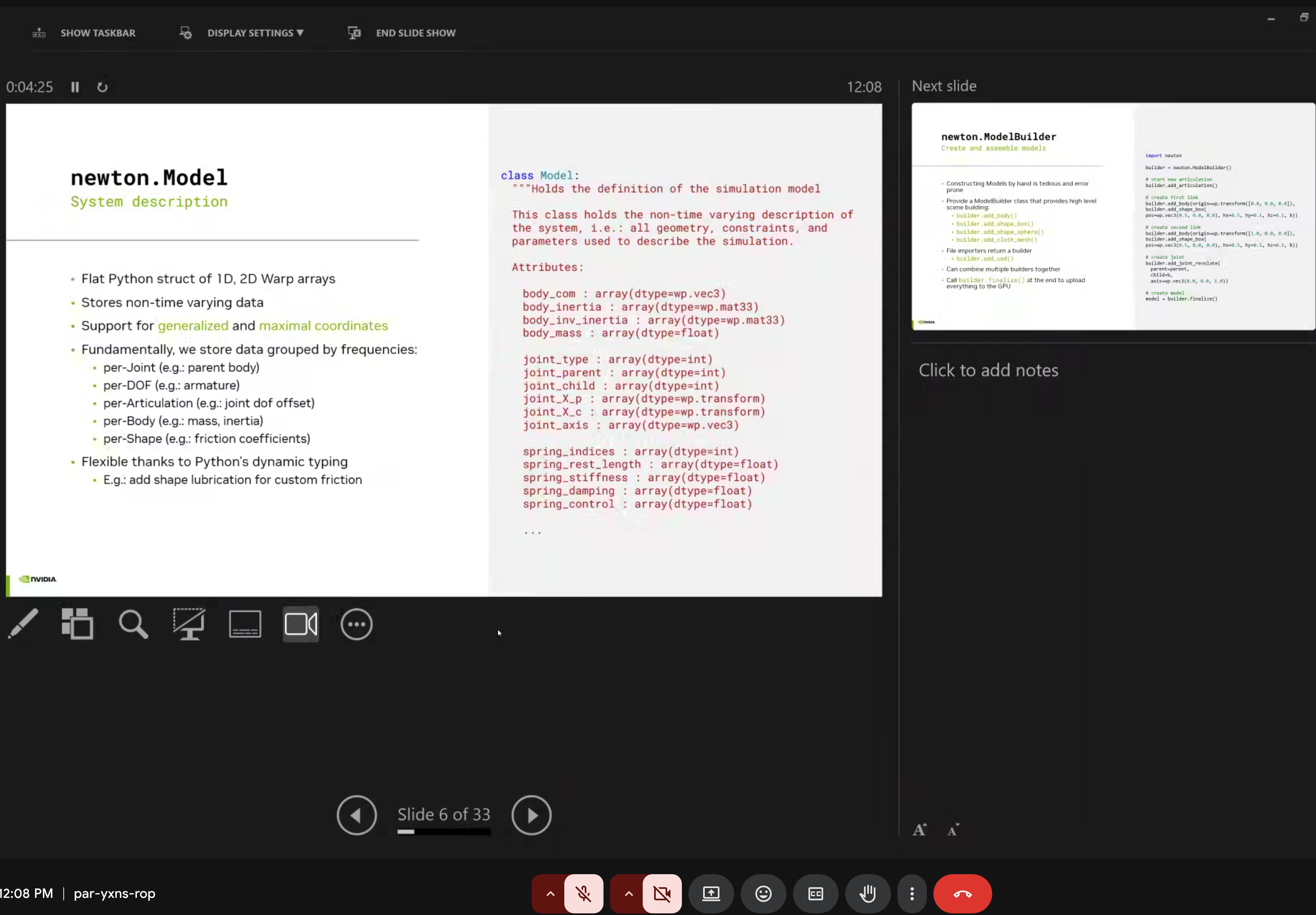
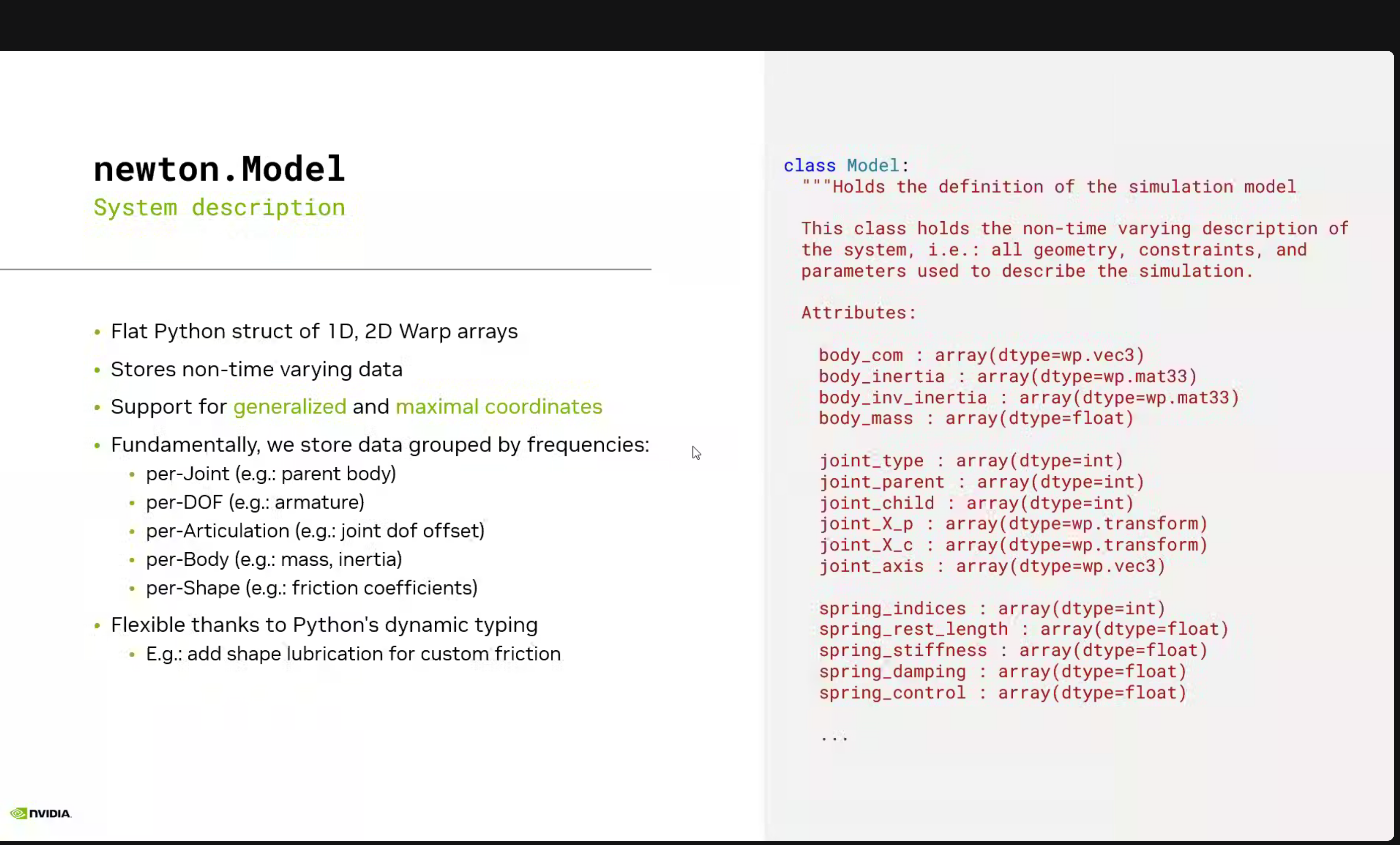
The newton.Model is a flat Python struct of 1D, 2D Warp arrays that stores non-time varying data, supporting generalized and maximal coordinates.
When working with Newton models, you might notice something surprising:
print(f"Bodies: {model.body_count}, Shapes: {model.shape_count}")
# Output: Bodies: 17, Shapes: 35  ← Why 35 shapes for 17 bodies?
Newton creates 2 shapes per body - one for visual geometry (rendering) and one for collision geometry (physics). This separation allows:
- Visual meshes to be high-detail (smooth rendering)
- Collision meshes to be simplified (fast physics)
To see which shape belongs to which body:
import numpy as np
shape_body = model.shape_body.numpy()  # Maps shape_idx → body_idx

for shape_idx, body_idx in enumerate(shape_body):
    print(f"Shape {shape_idx} → Body {body_idx}")
This is especially important when customizing colors with viewer.update_shape_colors() - you need to color all shapes, not just bodies! For a 17-body robot like the Go2-W, that’s 35 shape indices to consider (plus 1 for ground = 36 total).
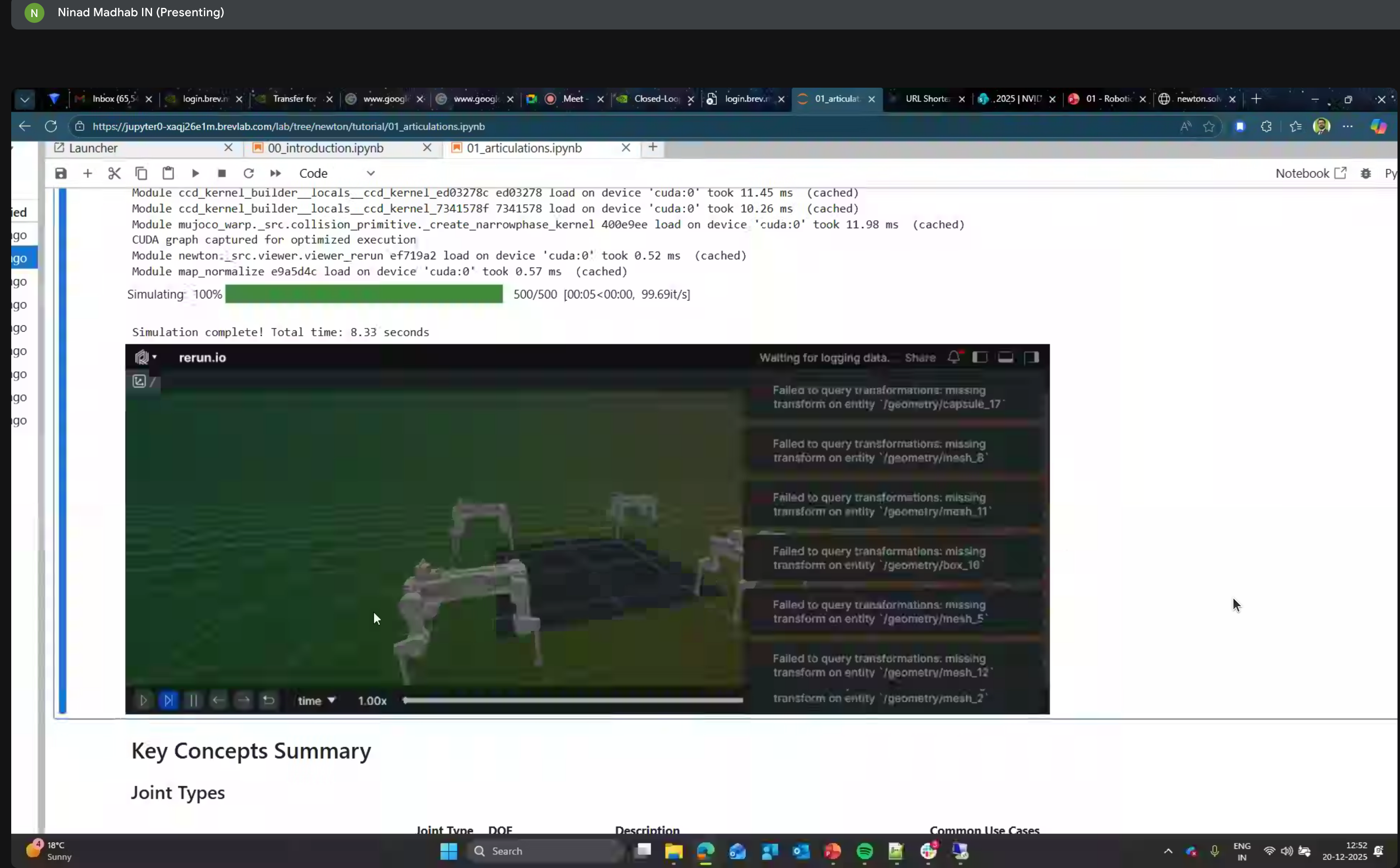
3. Articulations
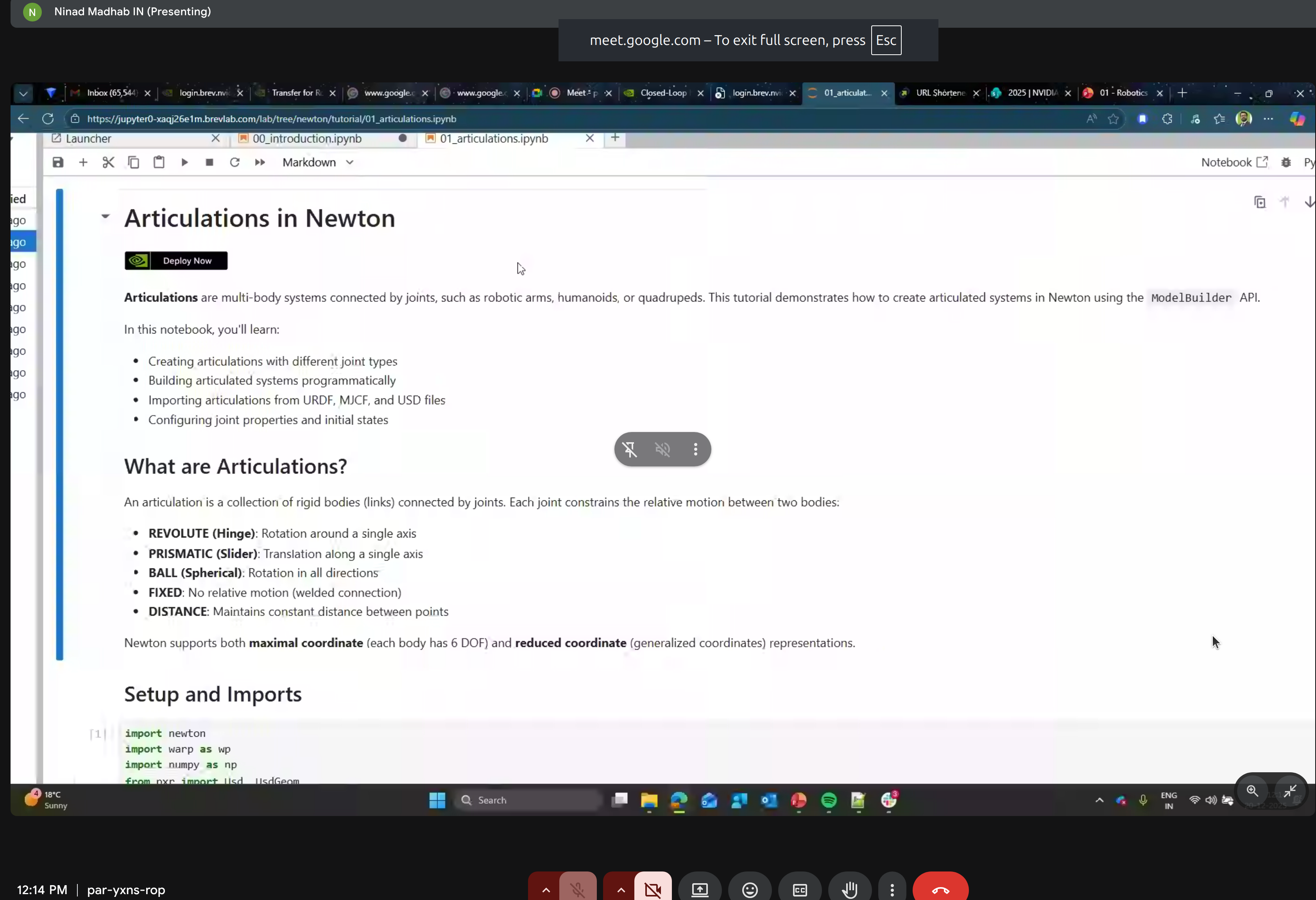
Multi-body systems connected by joints. Newton supports:
- REVOLUTE (Hinge) - Rotation around a single axis
- PRISMATIC (Slider) - Translation along a single axis
- BALL (Spherical) - Rotation in all directions
- FIXED - No relative motion (welded connection)
- DISTANCE - Maintains constant distance between points
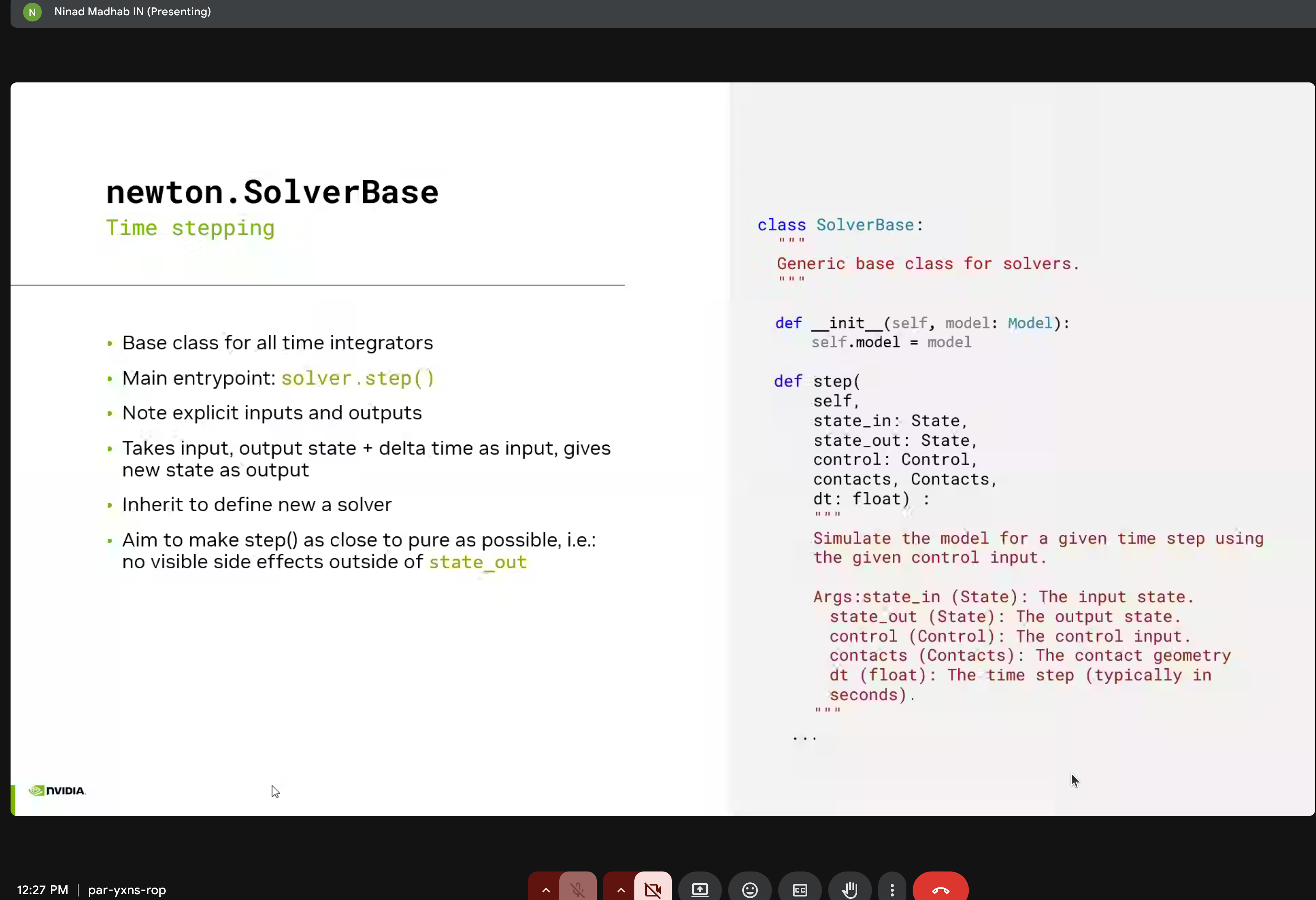
4. State Management
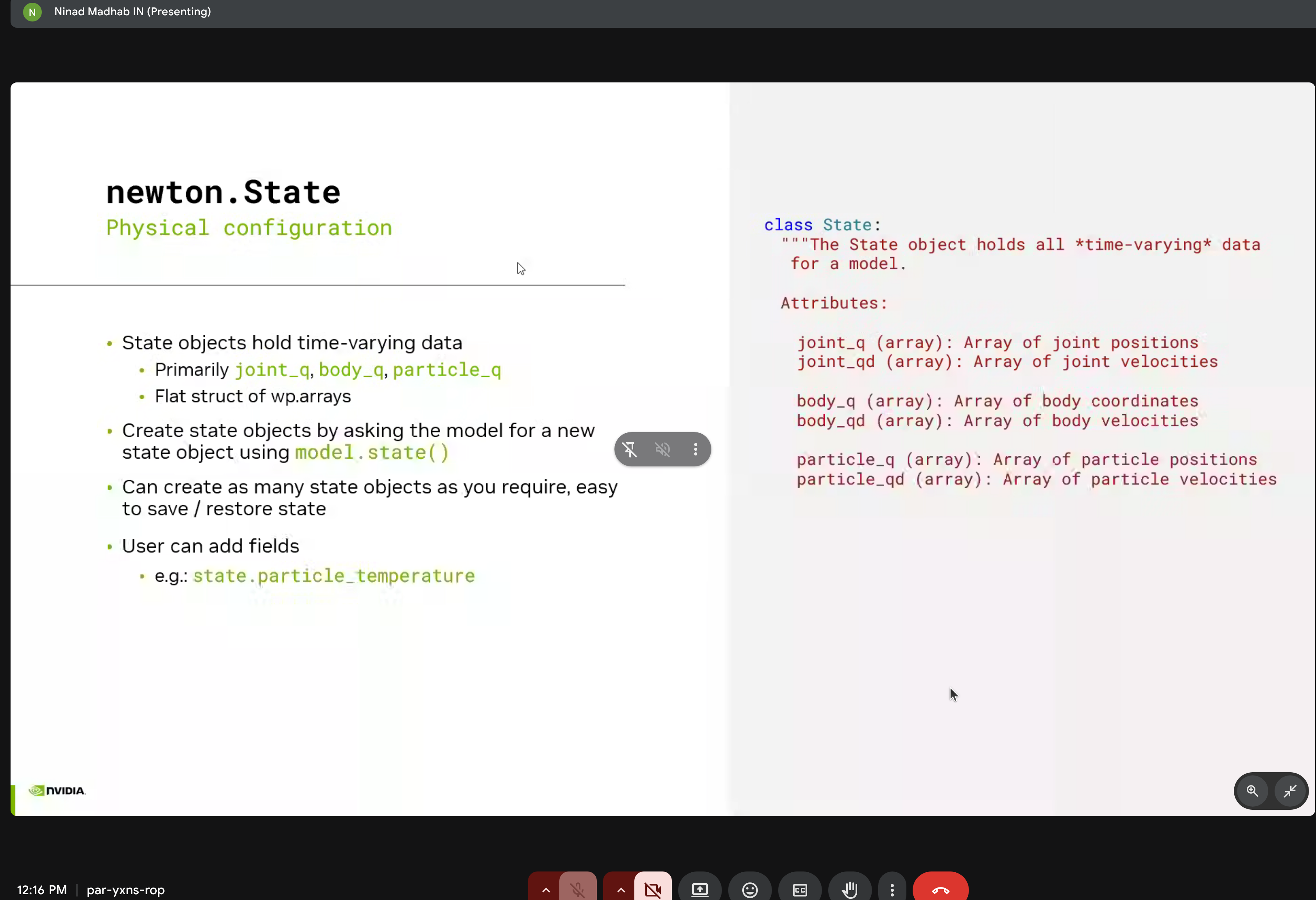
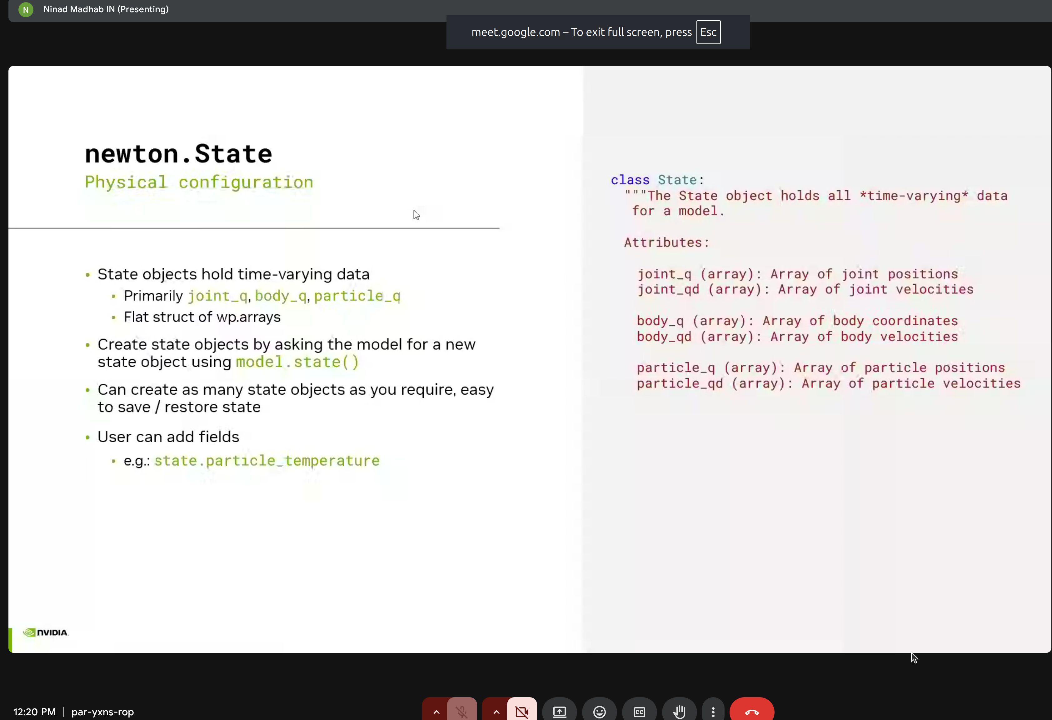
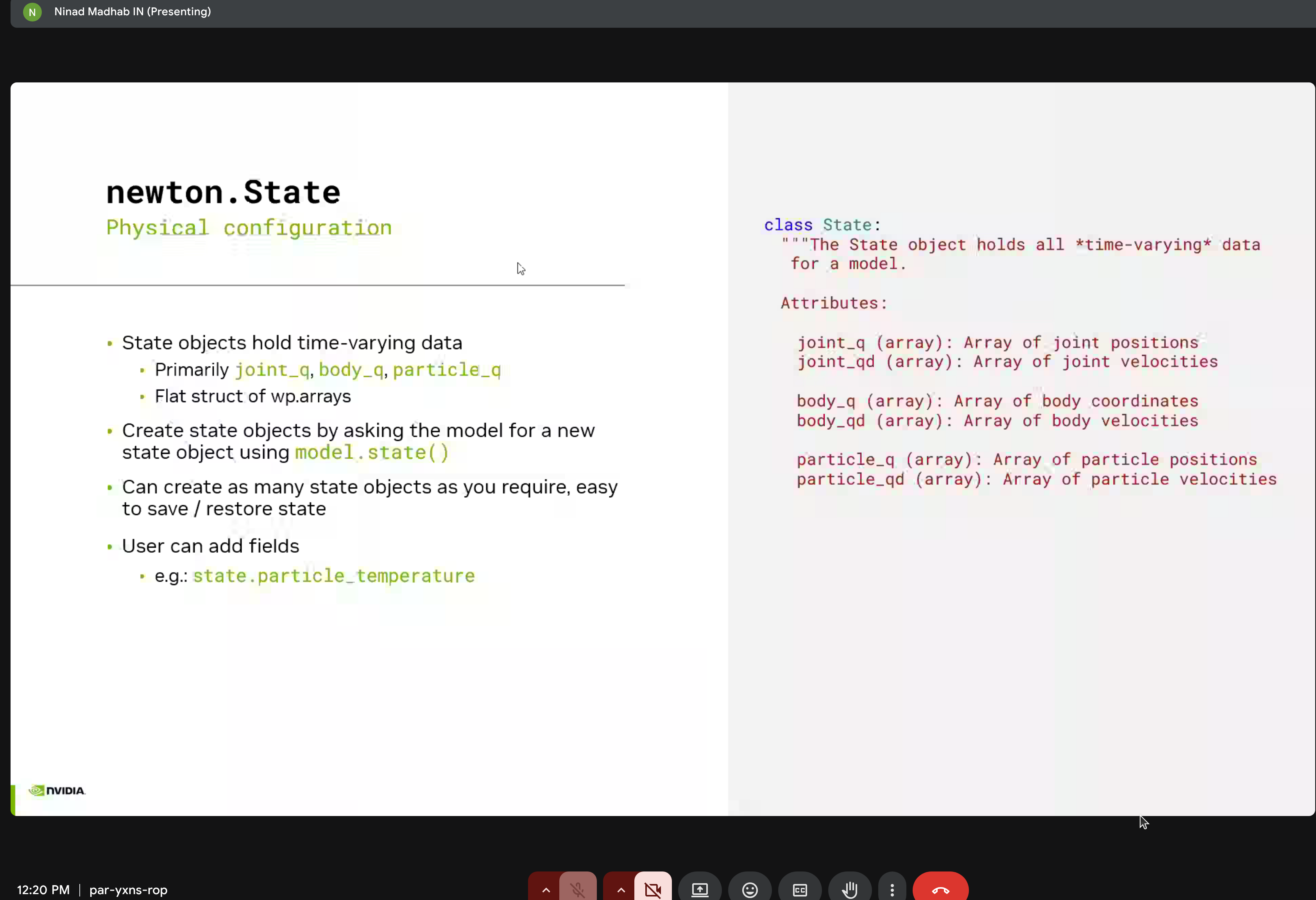
The newton.State class holds all time-varying simulation data:
class State:
    """Holds all time-varying data for a model."""

    # Joint state
    joint_q: wp.array   # Joint positions
    joint_qd: wp.array  # Joint velocities

    # Body state
    body_q: wp.array    # Body coordinates
    body_qd: wp.array   # Body velocities

    # Particle state
    particle_q: wp.array   # Particle positions
    particle_qd: wp.array  # Particle velocities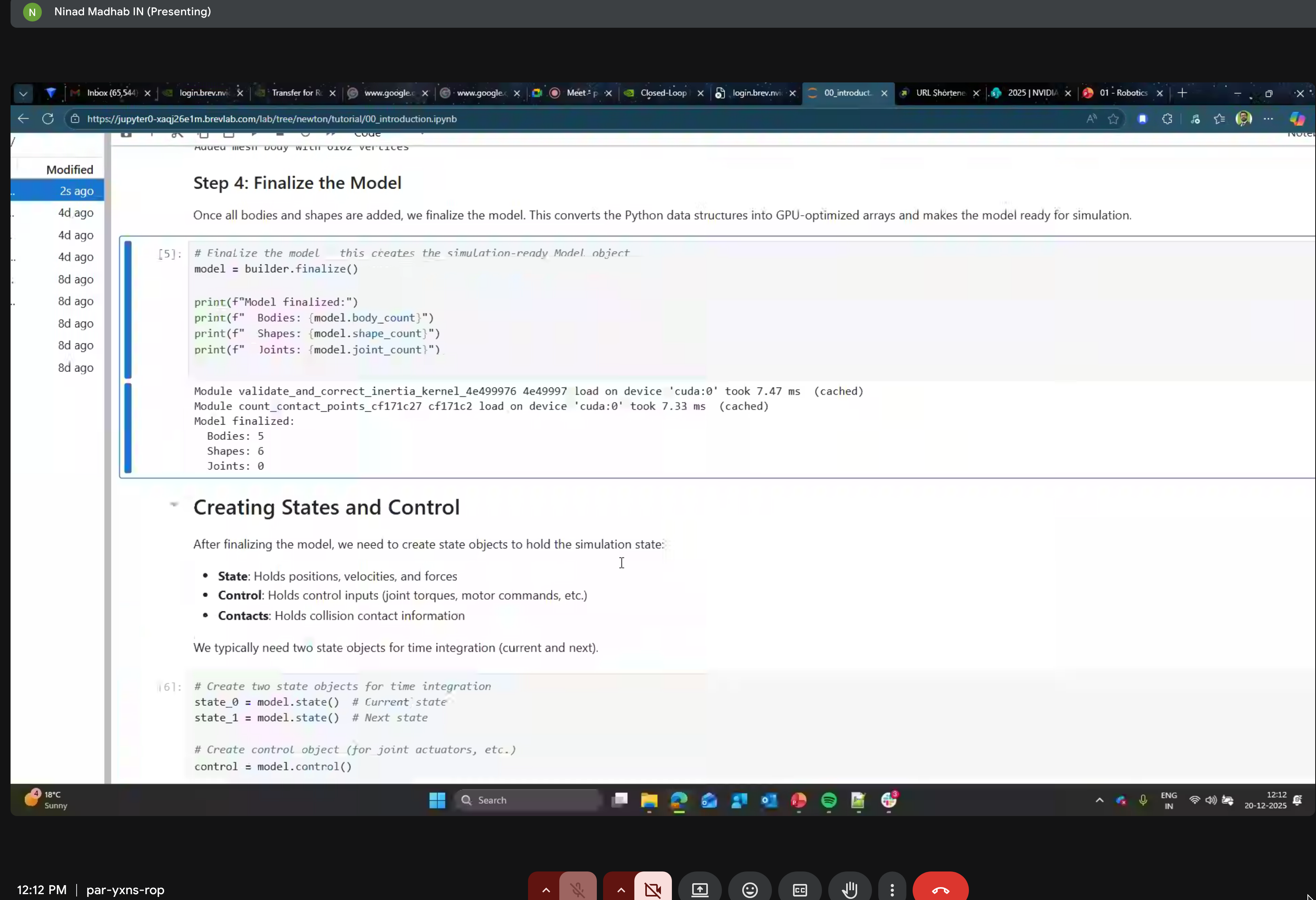
5. Control
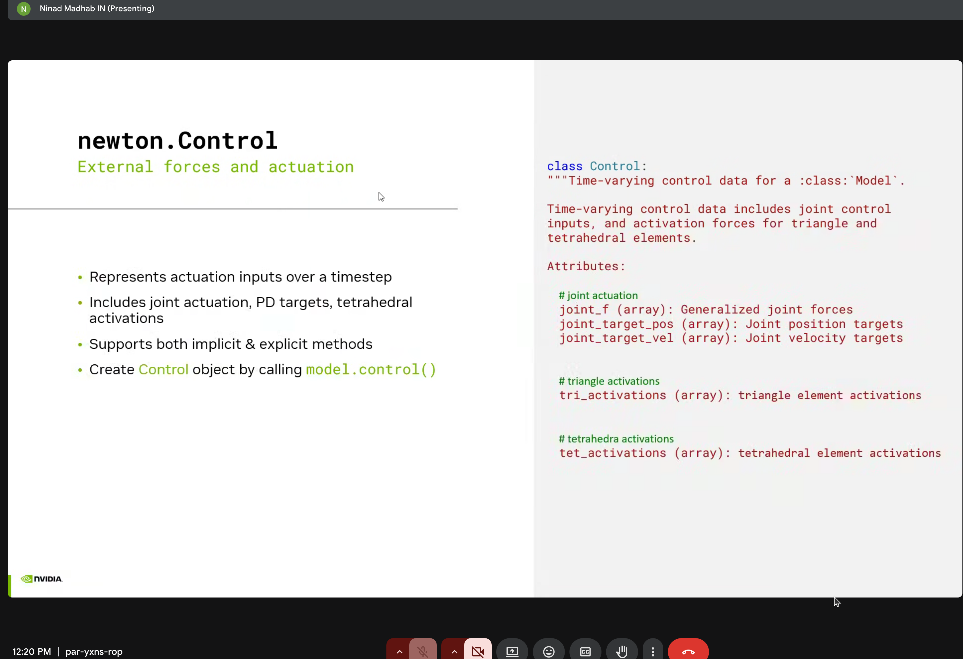
The newton.Control class manages external forces and actuation:
- Joint forces
- Position/velocity targets
- Triangle/tetrahedral element activations
6. Simulation Loop
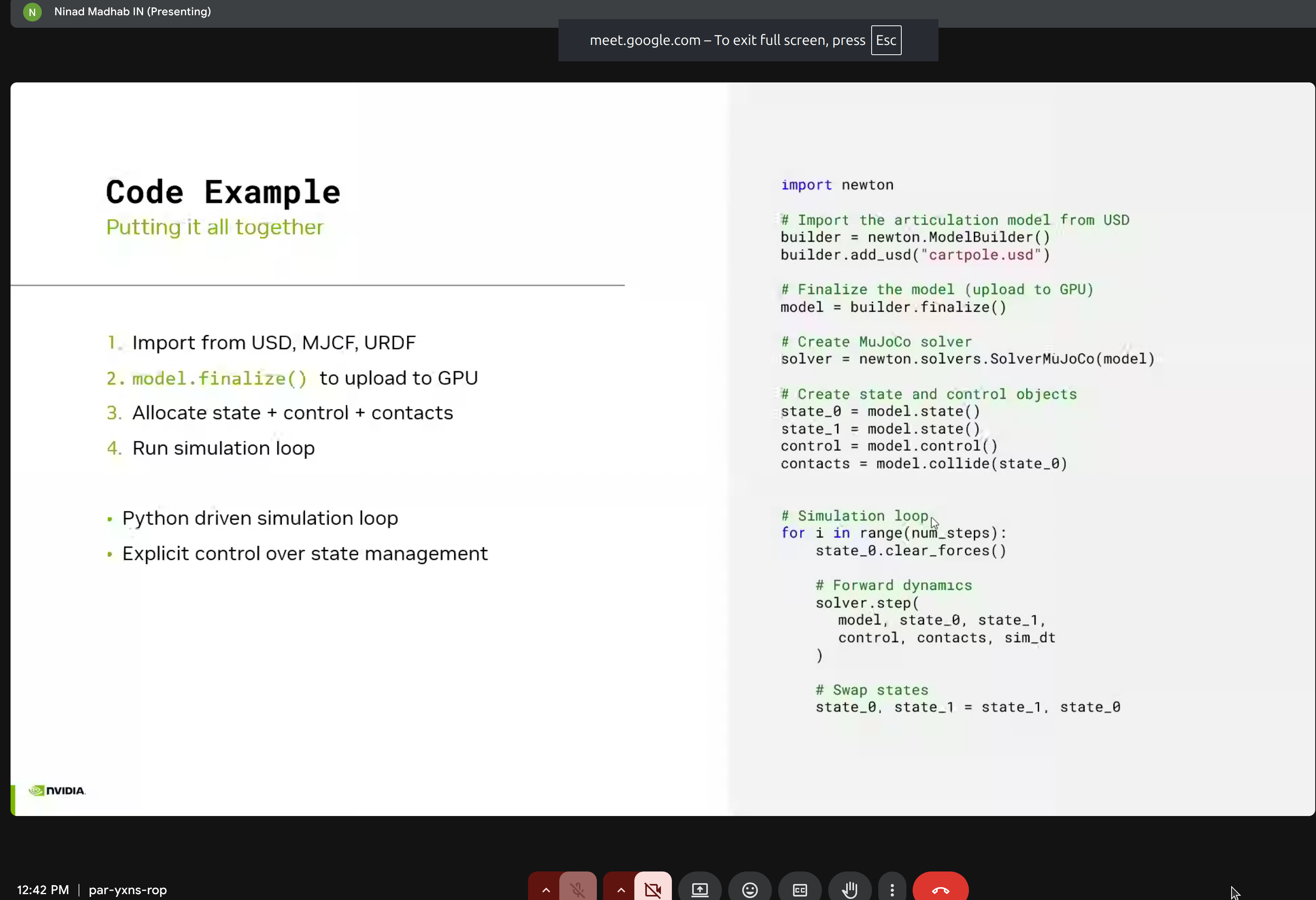
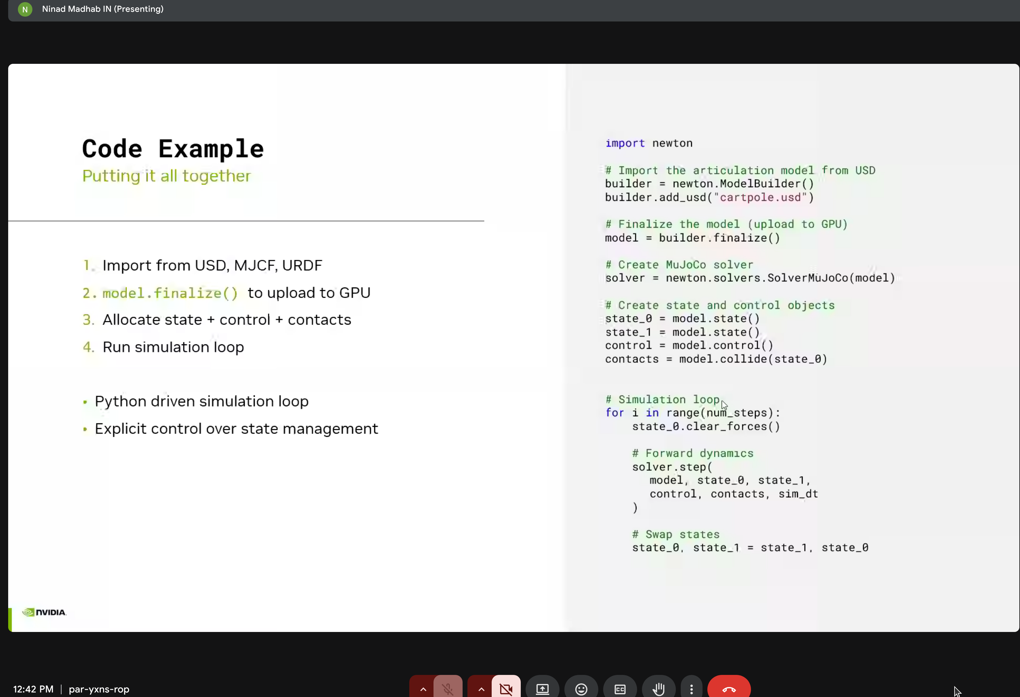
Putting it all together:
import newton
# Import model from USD
builder = newton.ModelBuilder()
builder.add_usd("cartpole.usd")
model = builder.finalize()
# Create MuJoCo solver
solver = newton.solvers.SolverMuJoCo(model)
# Create state and control objects
state_0 = model.state()
state_1 = model.state()
control = model.control()
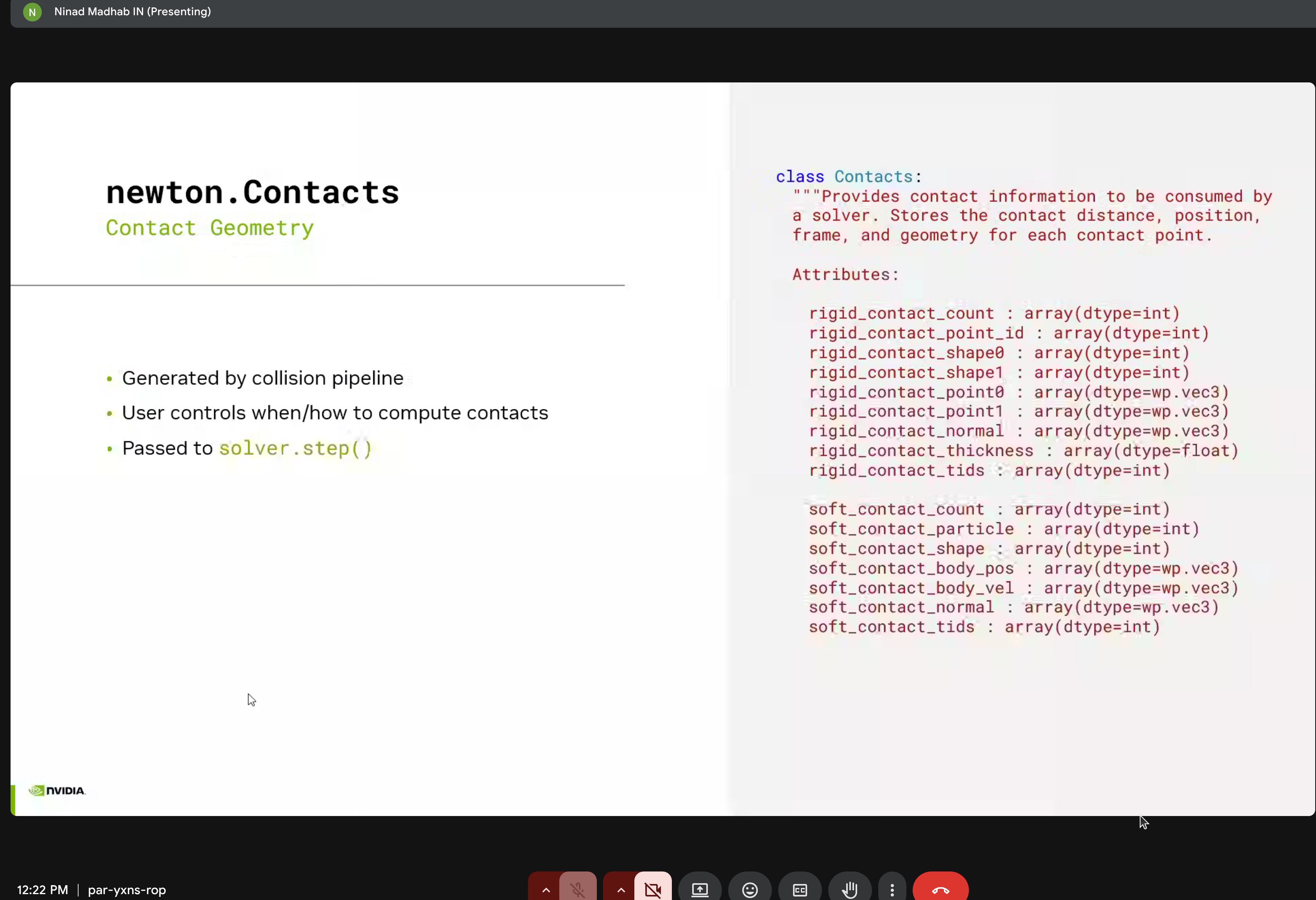
contacts = model.collide(state_0)
# Simulation loop
for i in range(num_steps):
state_0.clear_forces()
# Forward dynamics
solver.step(
model, state_0, state_1,
control, contacts, sim_dt
)
# Swap states
state_0, state_1 = state_1, state_0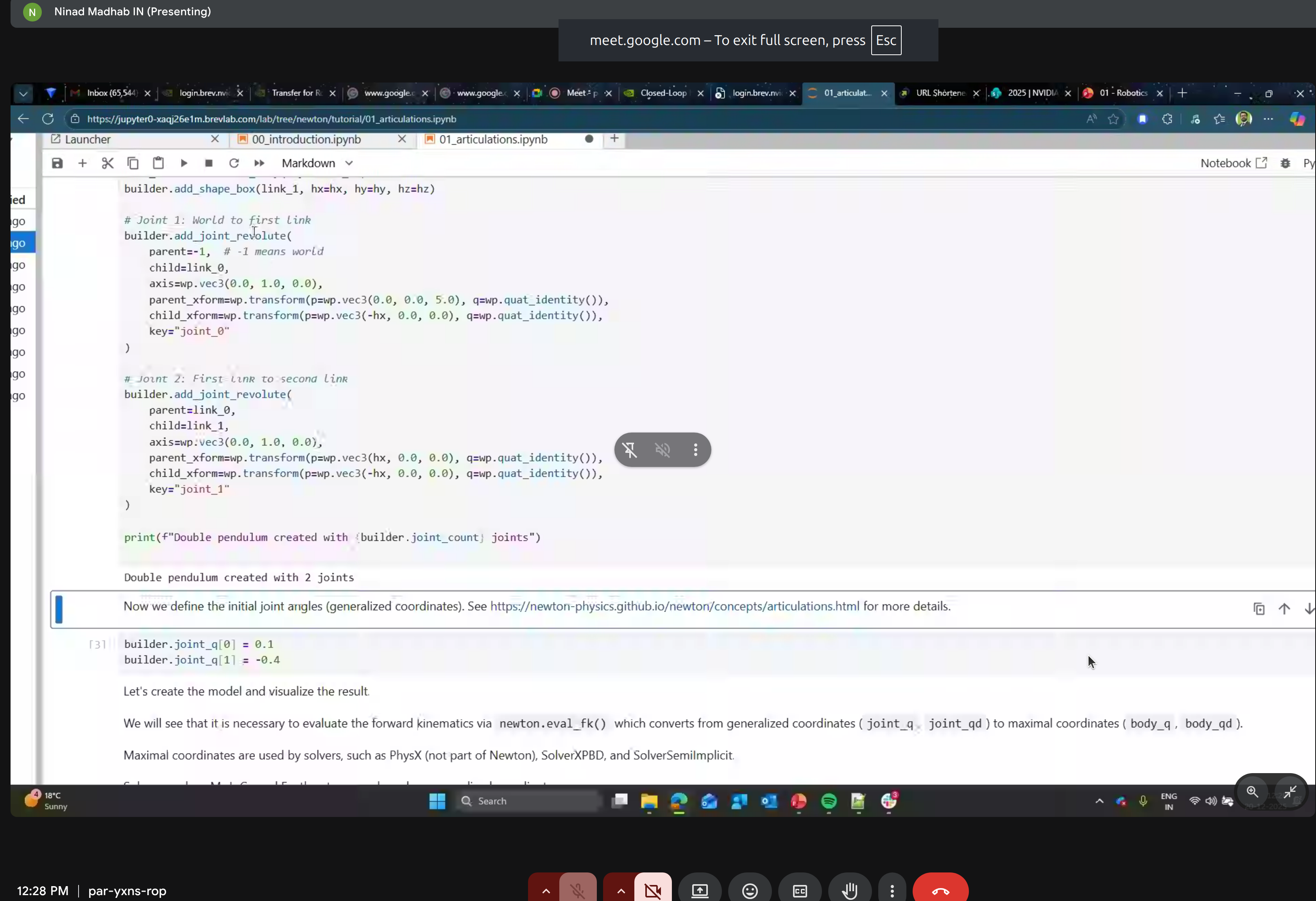
7. Solvers
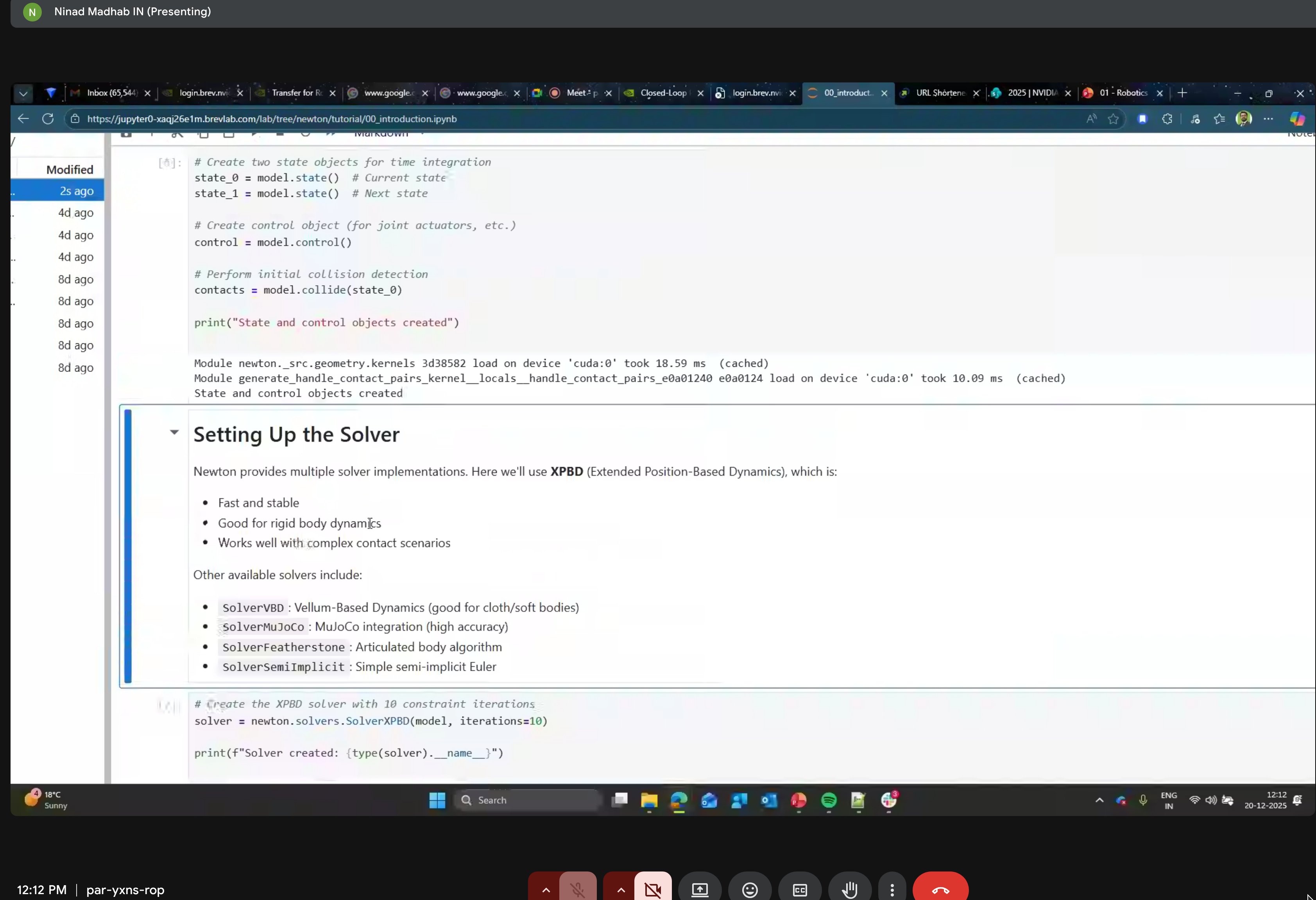
Newton provides multiple solver implementations:
- SolverXPBD - Extended Position Based Dynamics (fast, stable)
- SolverPBD - Position Based Dynamics
- SolverMuJoCo - MuJoCo-compatible solver
- SolverFeatherstone - Articulated body algorithm
- SolverSemiImplicit - Semi-implicit integration
8. GPU Acceleration with CUDA Graphs
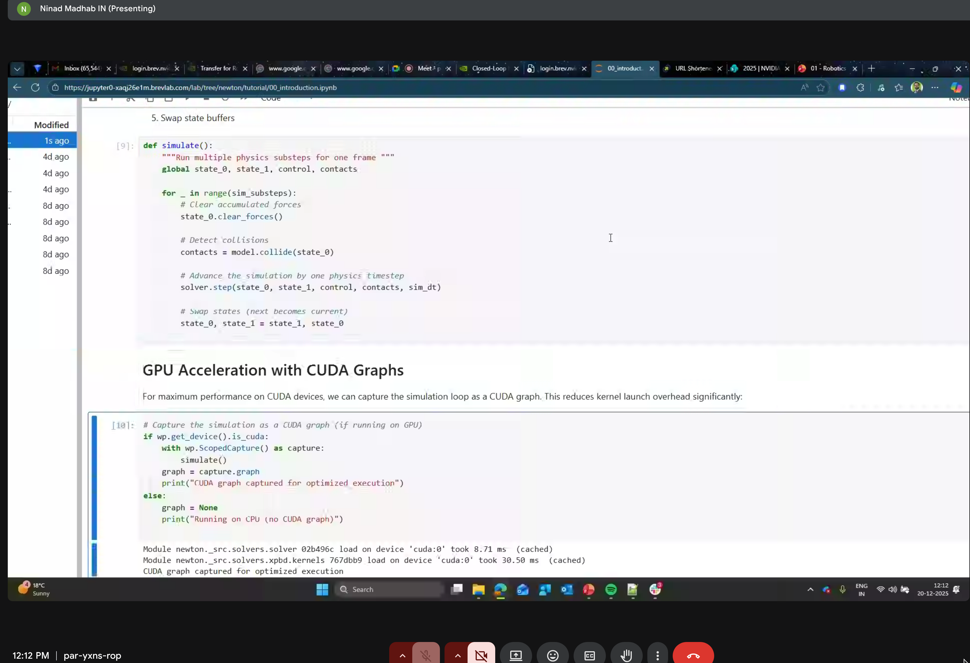
Reduce kernel launch overhead by capturing the simulation loop as a CUDA graph for optimized execution.
9. Selection API
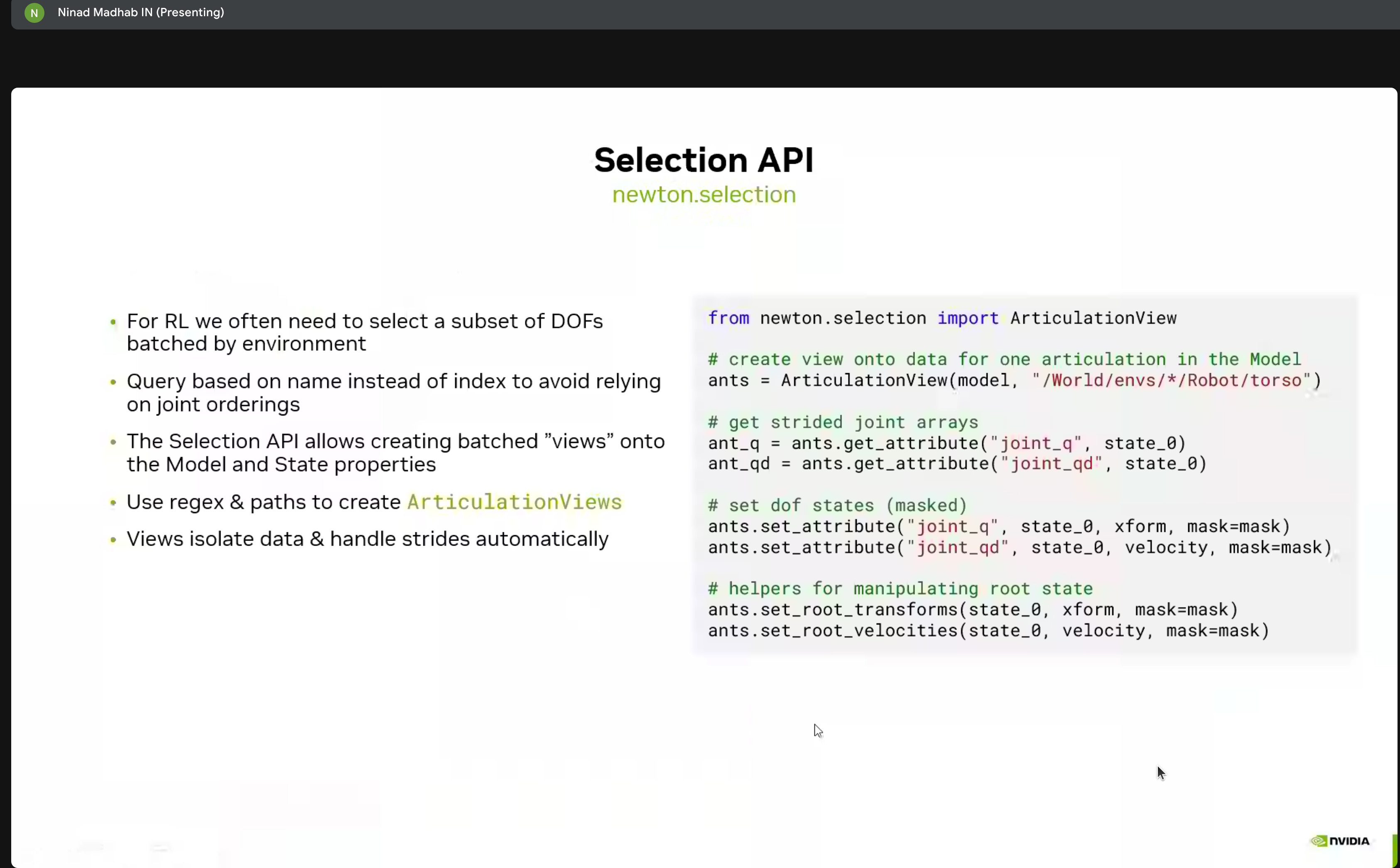
For reinforcement learning, we often need to select subsets of DOFs batched by environment:
from newton.selection import ArticulationView

# Create view onto data for one articulation
ants = ArticulationView(model, "/World/envs/*/Robot/torso")

# Get strided joint arrays
ant_q = ants.get_attribute("joint_q", state_0)
ant_qd = ants.get_attribute("joint_qd", state_0)

# Set DOF states (masked)
ants.set_attribute("joint_q", state_0, xform, mask=mask)
ants.set_attribute("joint_qd", state_0, velocity, mask=mask)

# Helpers for manipulating root state
ants.set_root_transforms(state_0, xform, mask=mask)
ants.set_root_velocities(state_0, velocity, mask=mask)
Geometry & Contacts
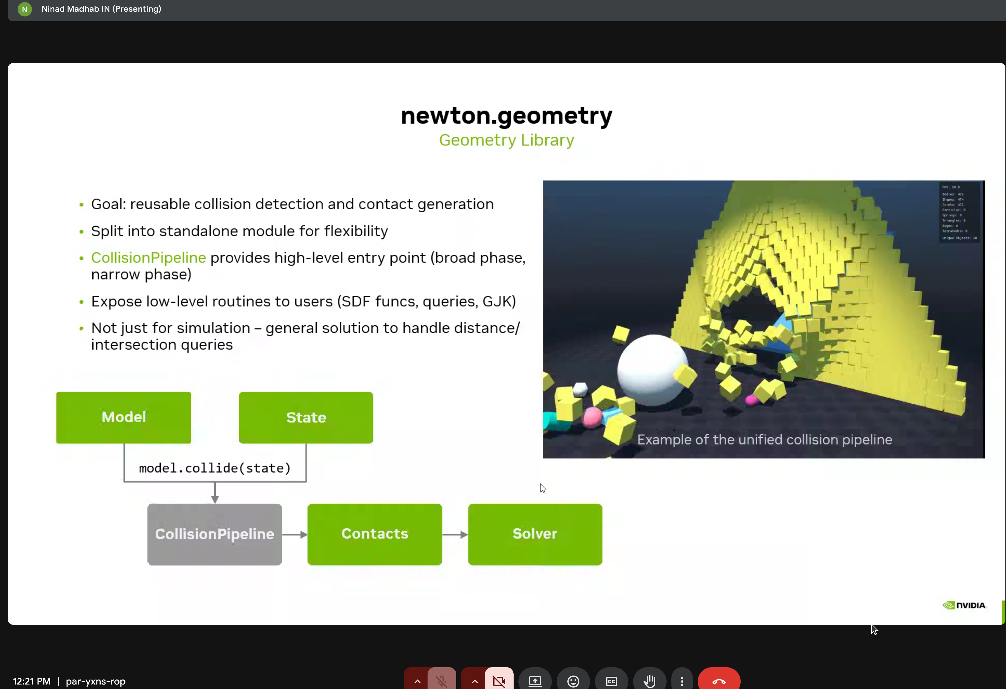
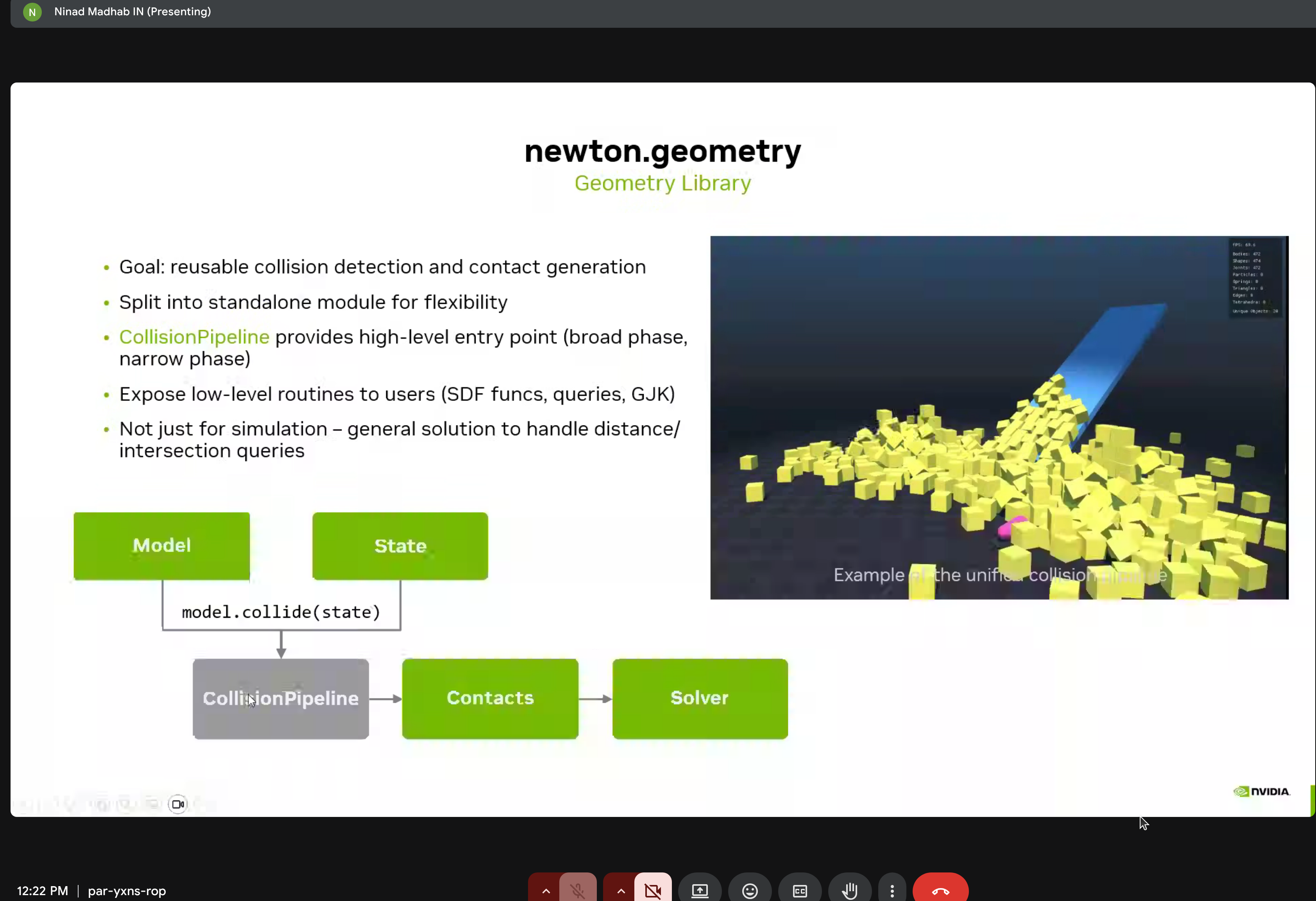
Newton includes sophisticated contact modeling via newton.geometry:
- SDF-SDF collision detection with multi-stage broadphase and narrow-band SDFs
- Meshes are converted to narrow-band SDFs
- Contact constraints generated from isosurface triangles
- Area-dependent scaling of MuJoCo constraint parameters
- Contact reduction finds representative points from thousands of generated contacts
Hydroelastic Contacts
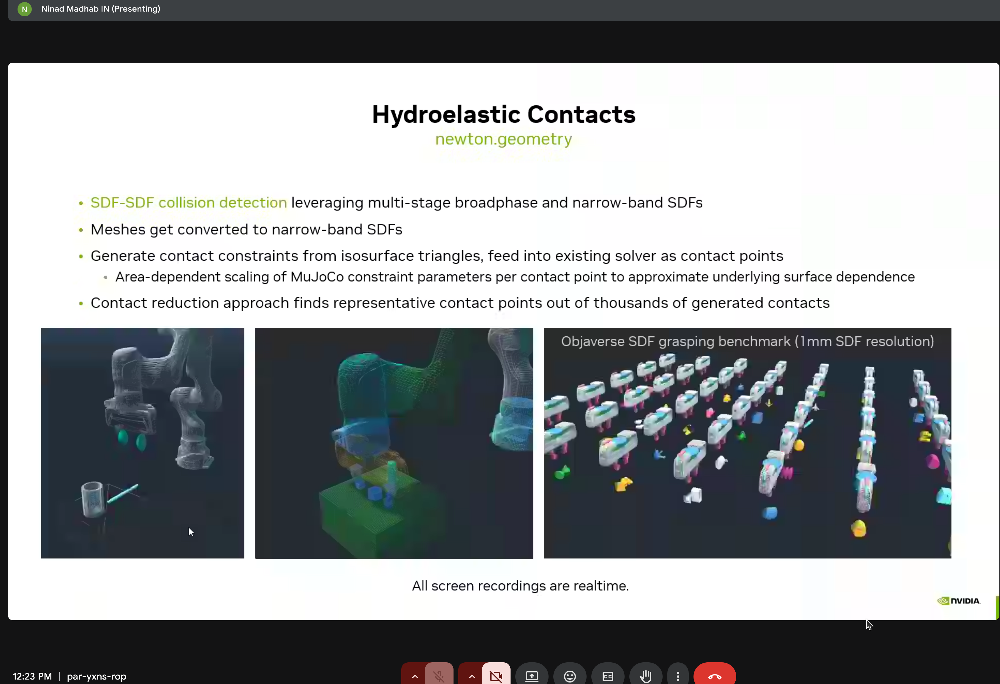
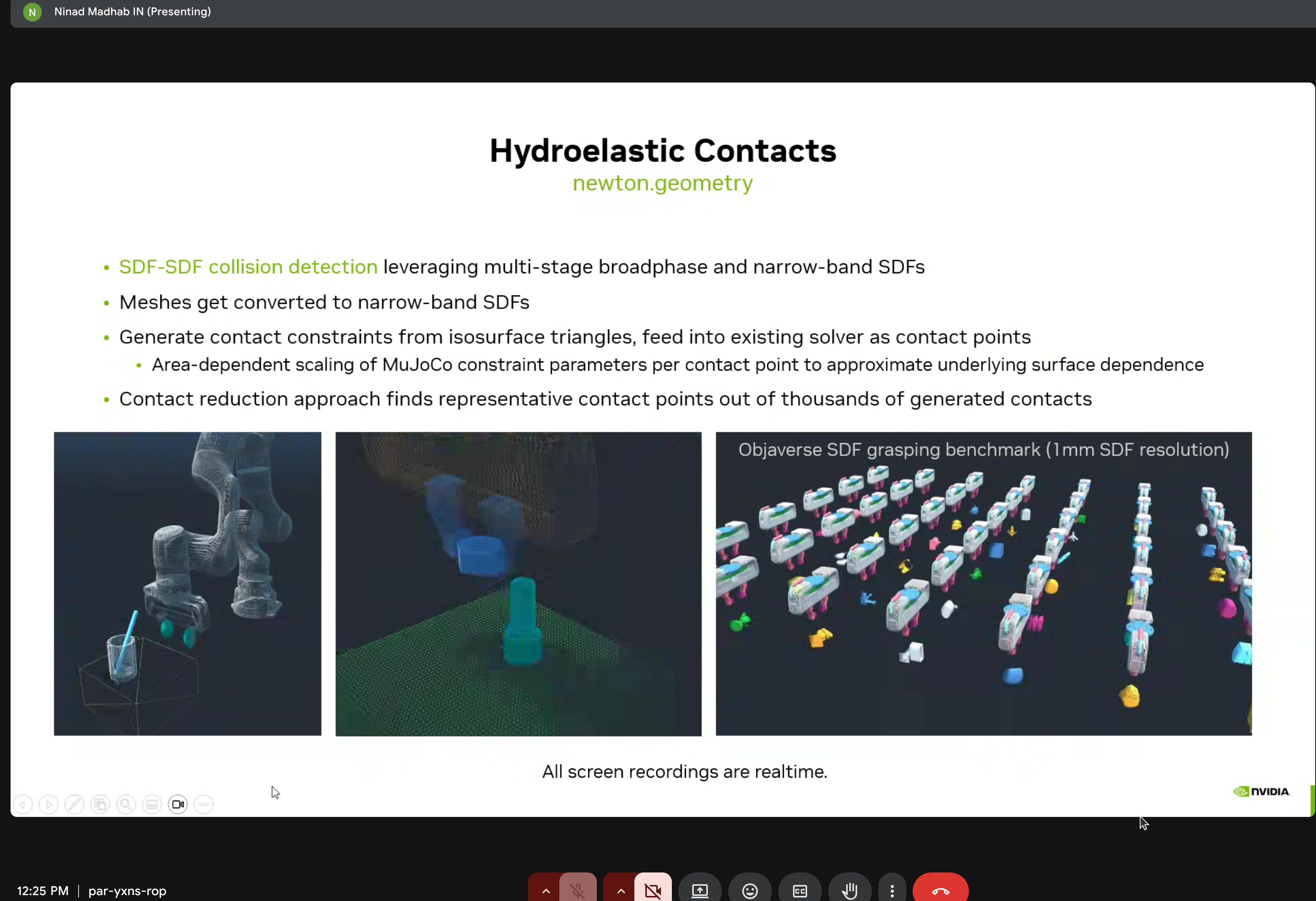
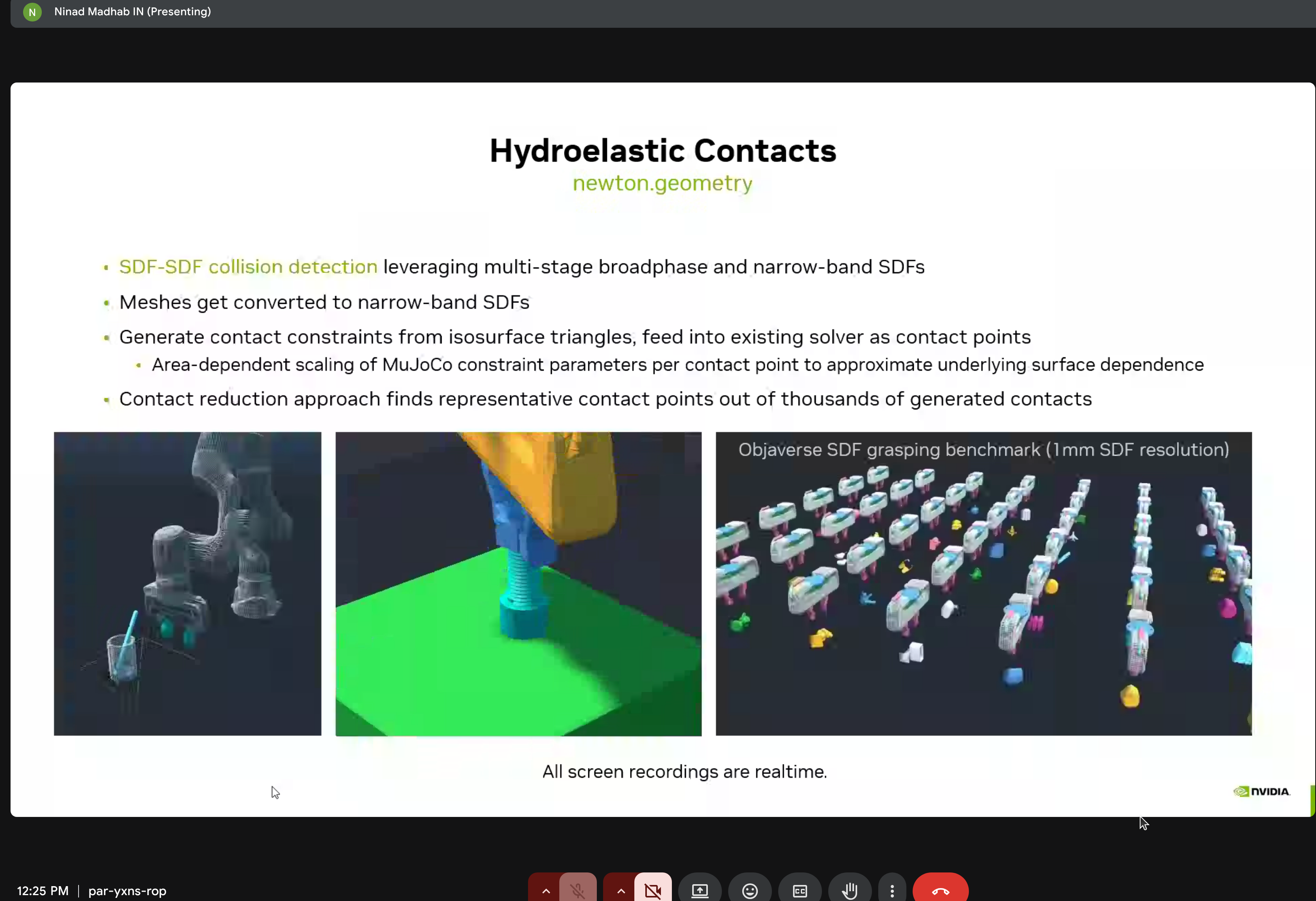
The demo showed the Objaverse SDF grasping benchmark at 1mm SDF resolution - all running in realtime!
Advanced Solvers
MuJoCo Solver Performance
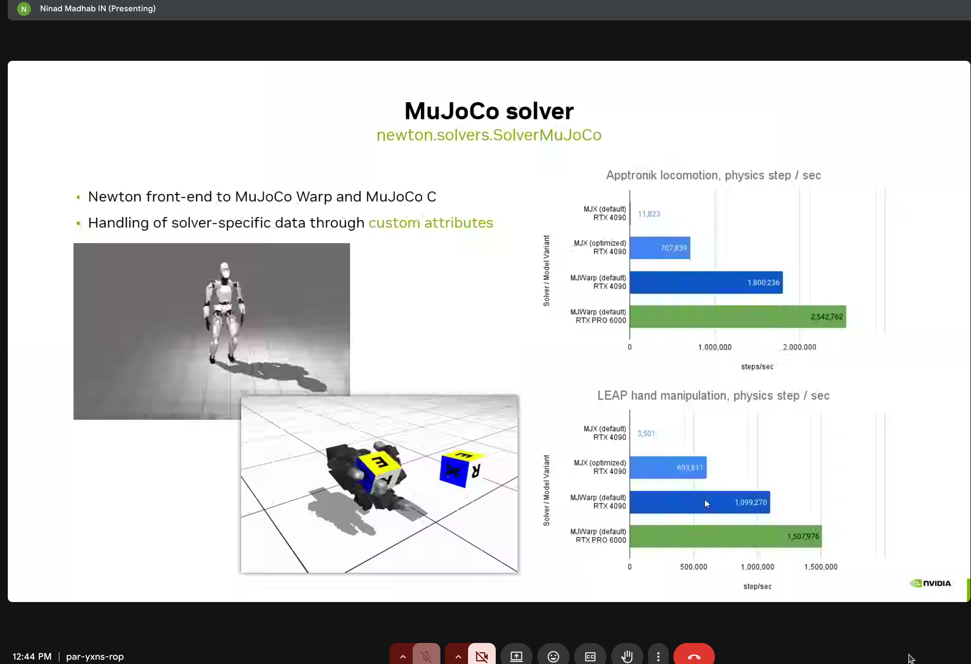
Performance comparisons for Apptronk locomotion and LEAP hand manipulation on RTX 6000.
VBD Solver for Cloth
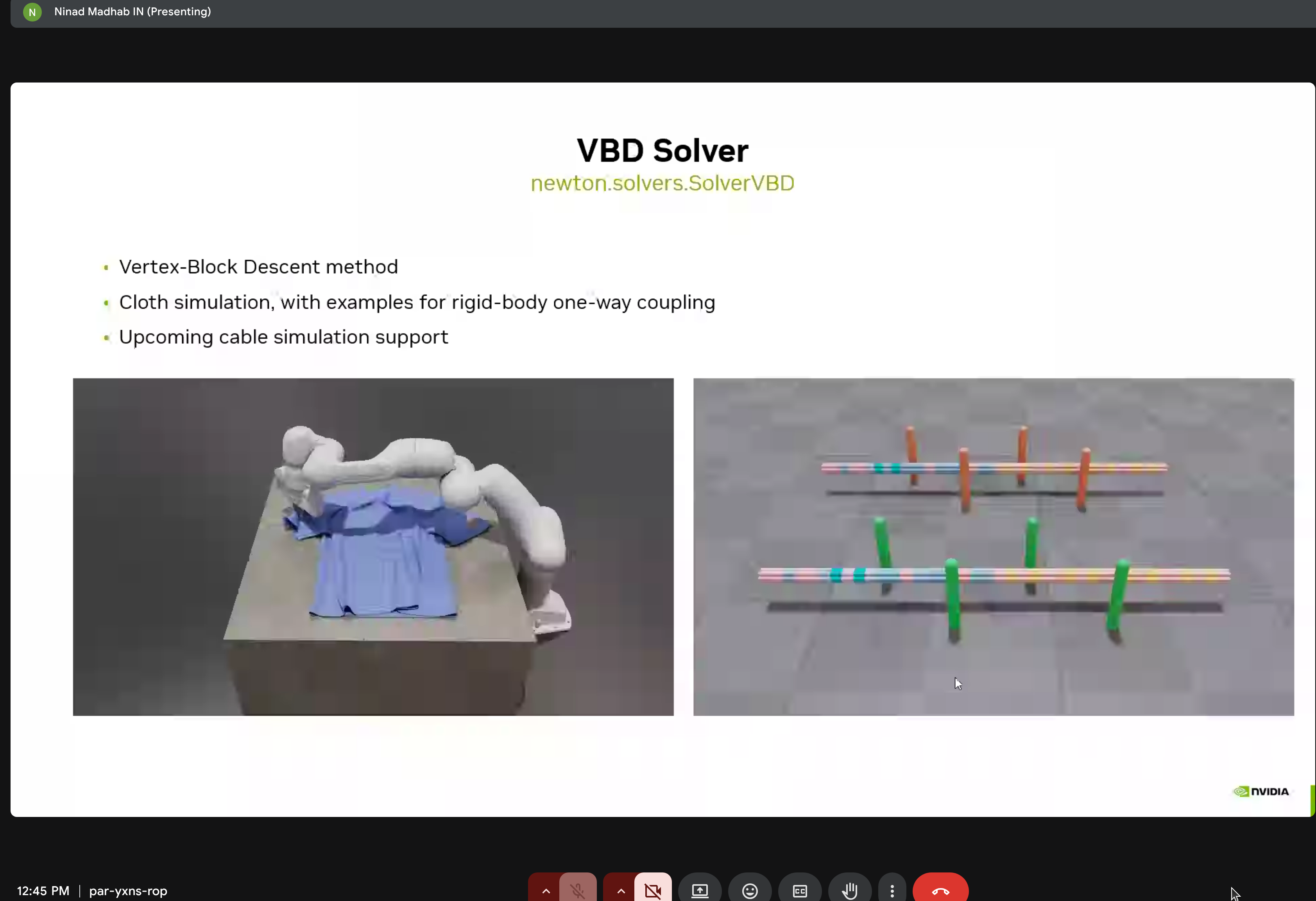
Vertex-Block Descent method with rigid-body one-way coupling and upcoming cable simulation support.
MPM Solver for Granular Materials
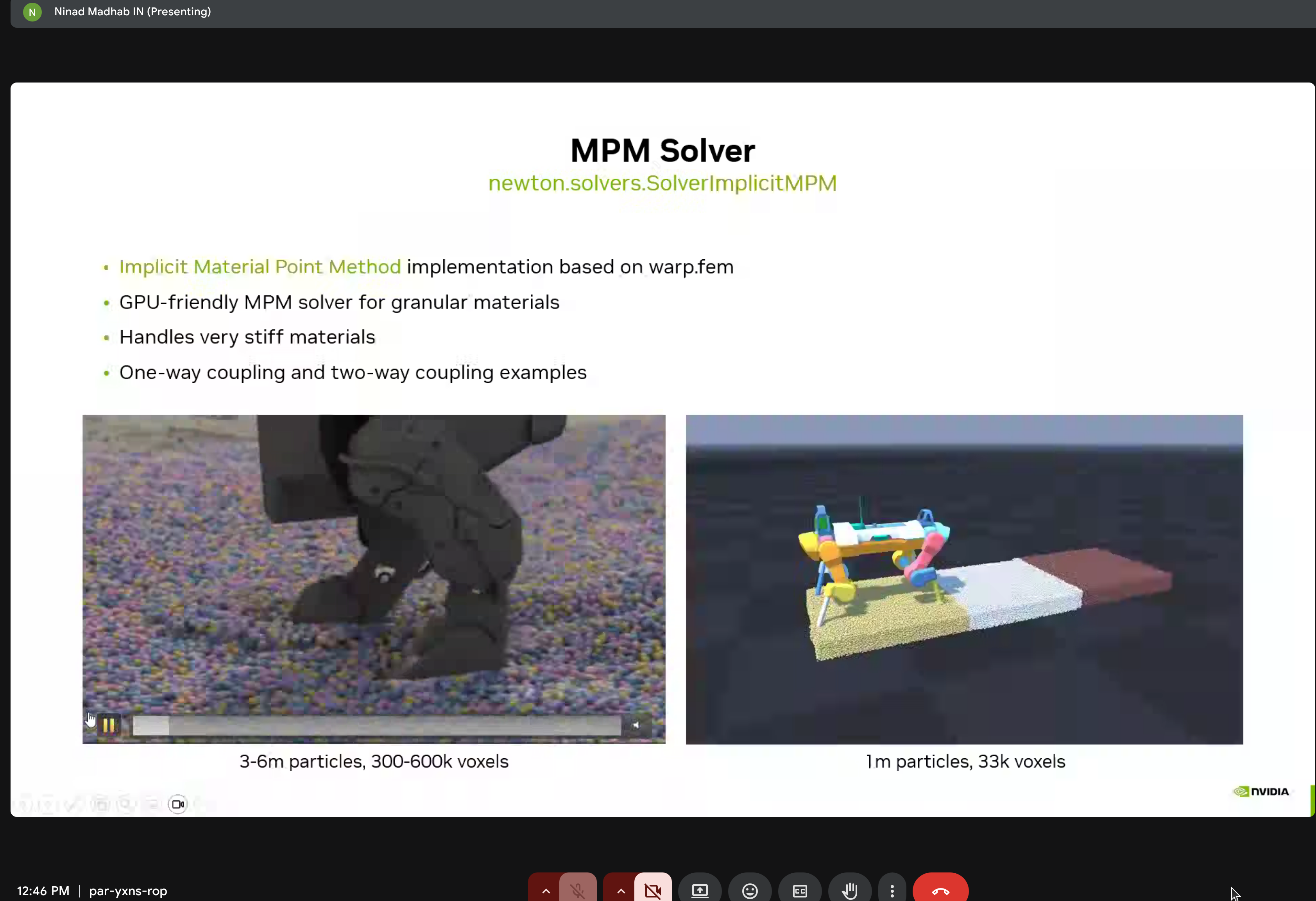
Implicit MPM implementation based on warp.fem - GPU-friendly solver for granular materials handling very stiff materials.
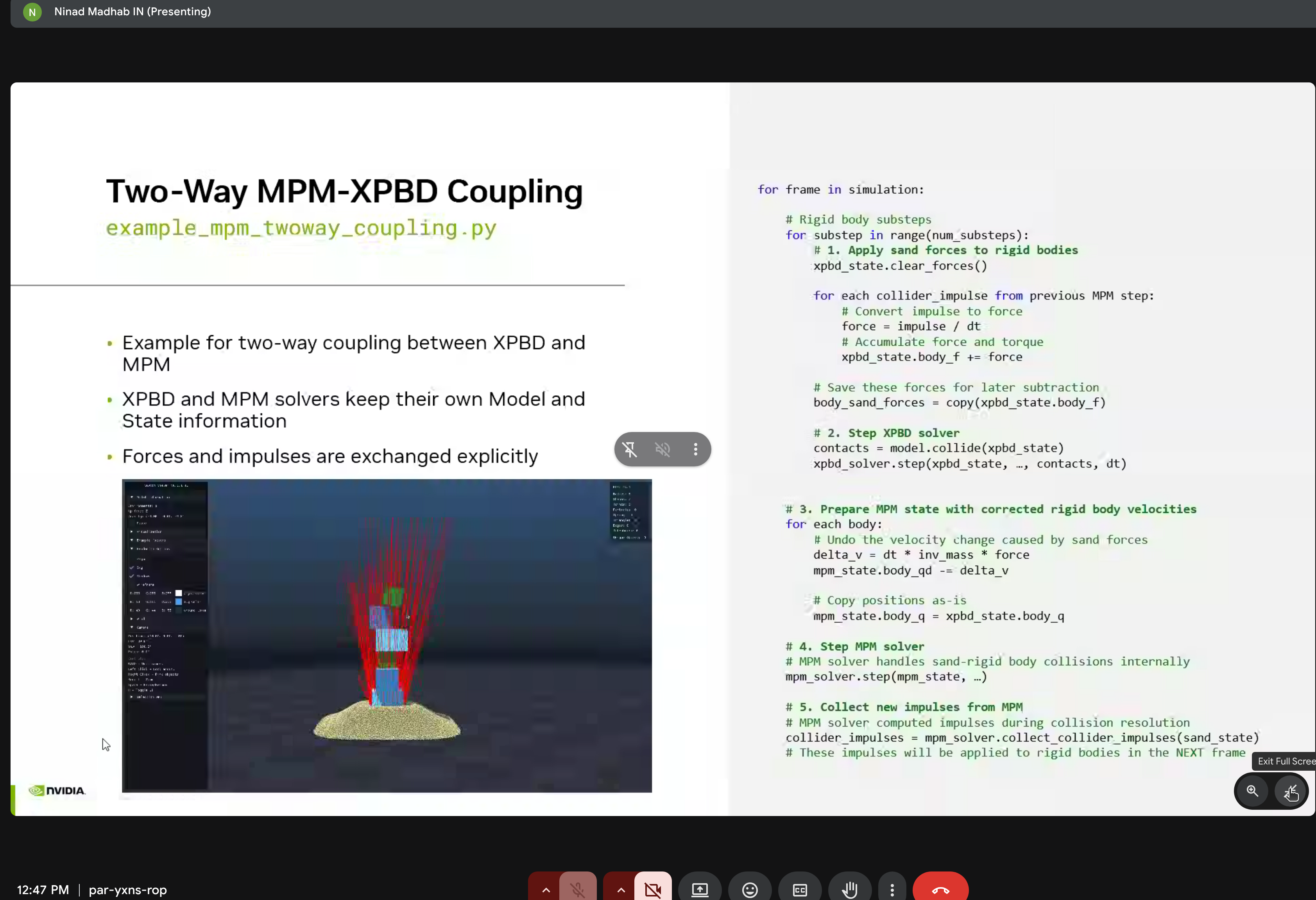
Two-way coupling where XPBD and MPM solvers exchange forces and impulses explicitly.
Inverse Kinematics
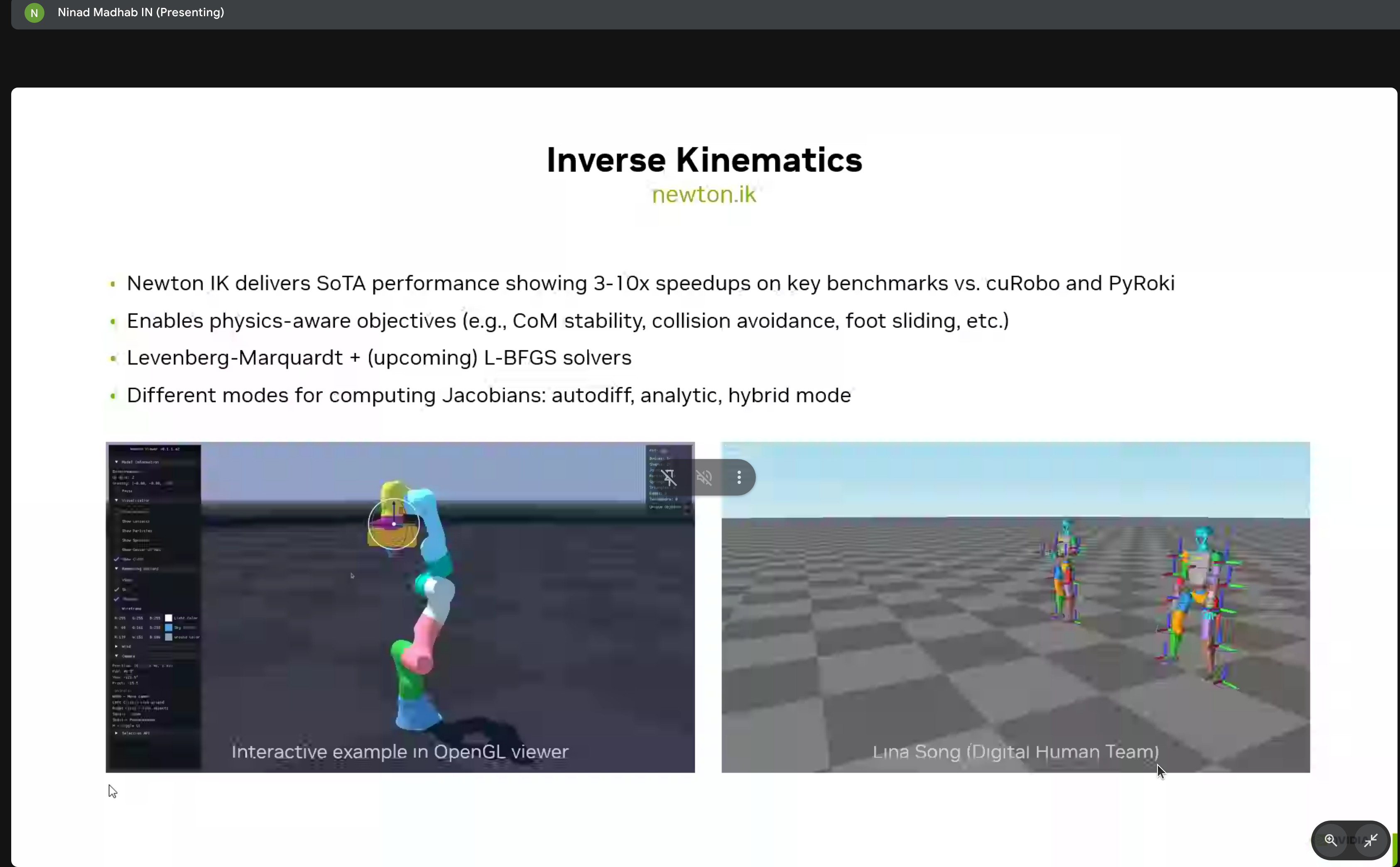
Newton’s IK module provides 3-10x speedups over cuRobo and PyRoki with:
- Physics-aware objectives
- Levenberg-Marquardt and L-BFGS solvers
- Interactive OpenGL viewer
Sensors
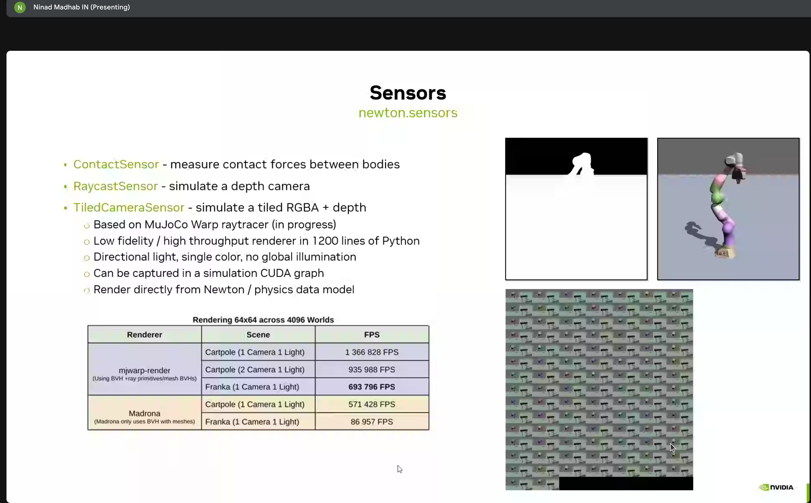
Newton includes various sensor types:
- ContactSensor - Contact force sensing
- RaycastSensor - Lidar-style raycasting
- TiledCameraSensor - Depth camera simulation
Custom Attributes & Extensions
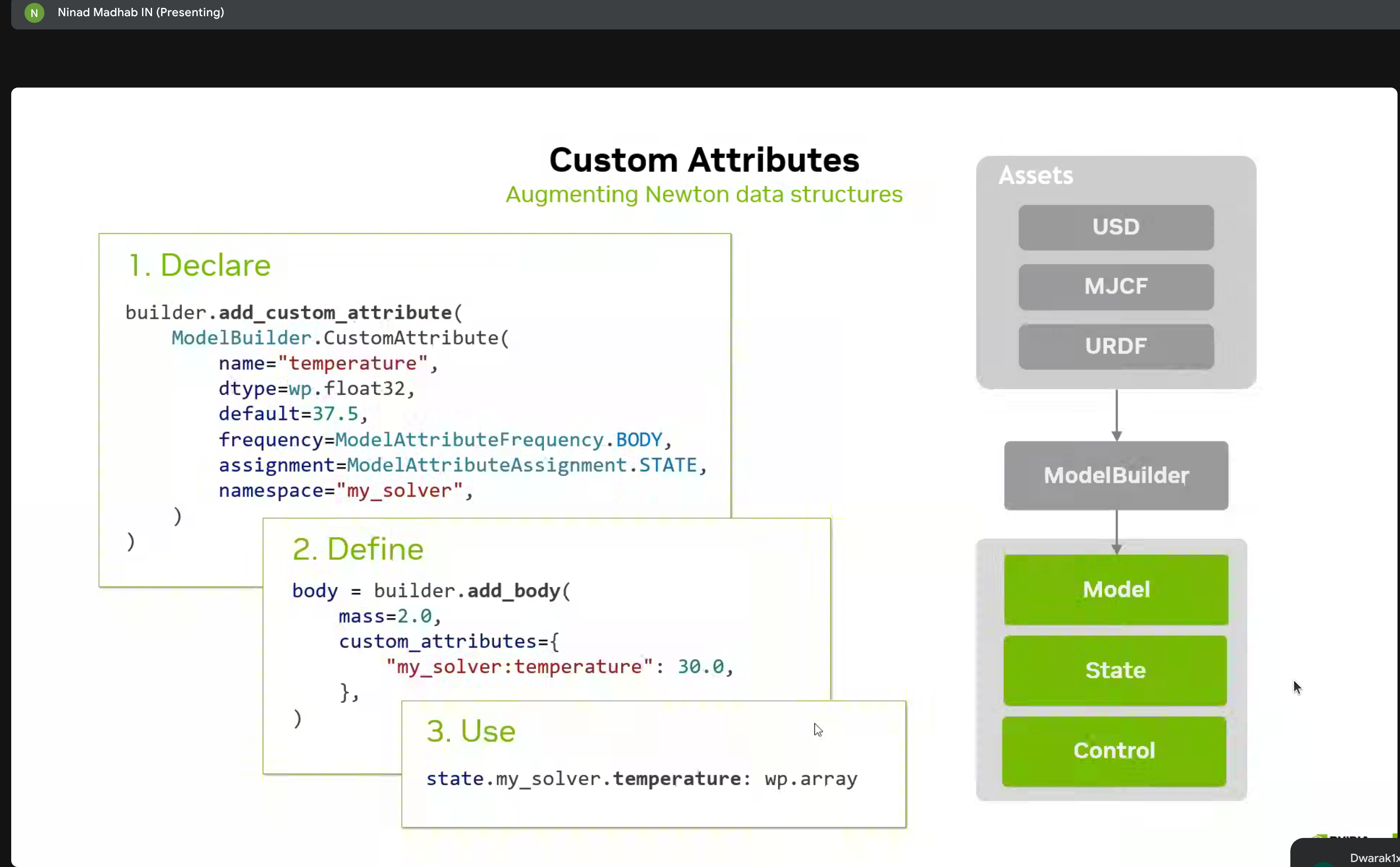
Three-step process for augmenting Newton data structures:
- Declare - Define custom properties
- Define - Implement behavior
- Use - Access in simulation
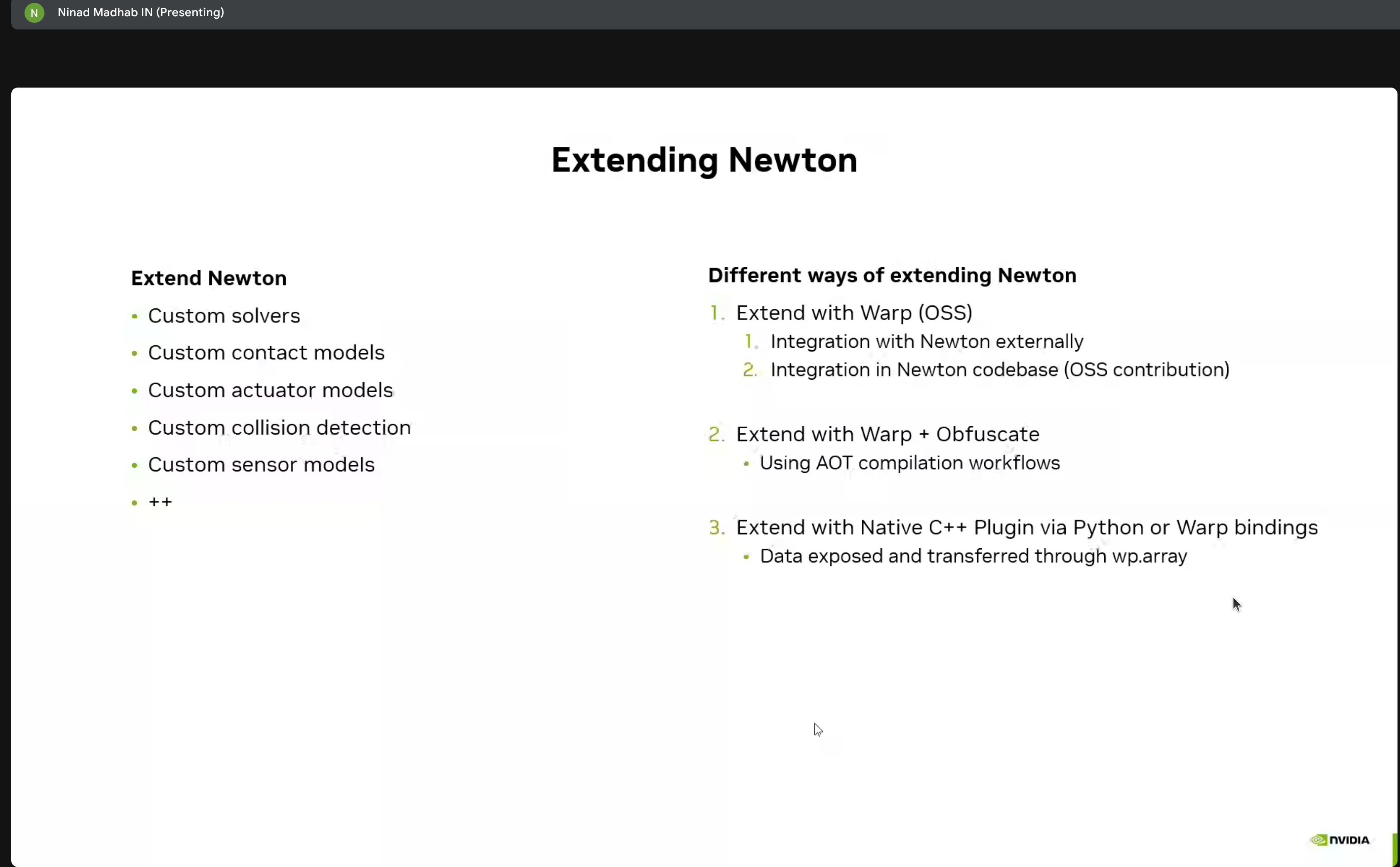
Multiple methods for extending Newton:
- Custom solvers
- Contact models
- Integration with Warp and C++ plugins
Hands-on Lab Environment
The workshop used Brev.dev for cloud-based GPU access:
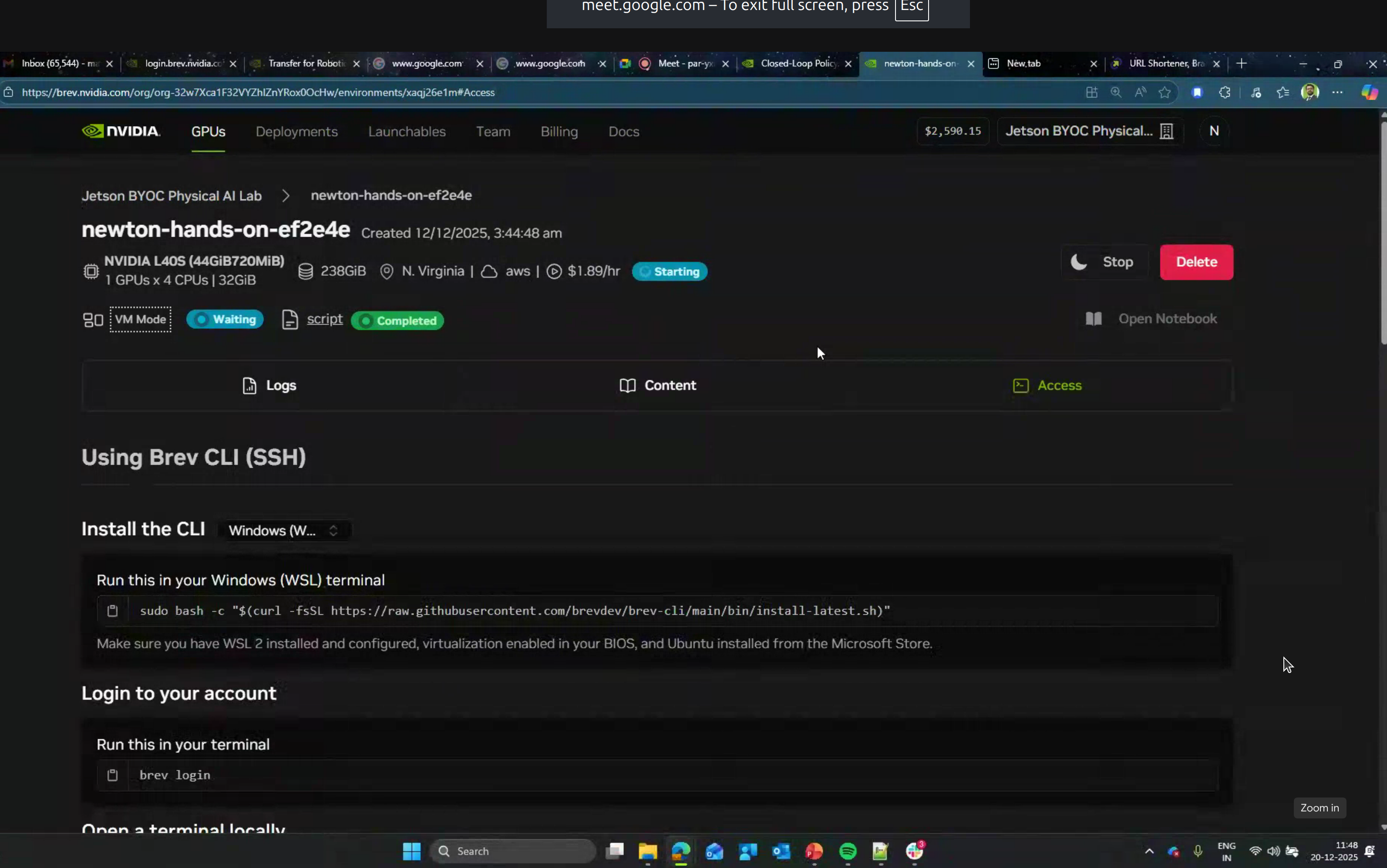
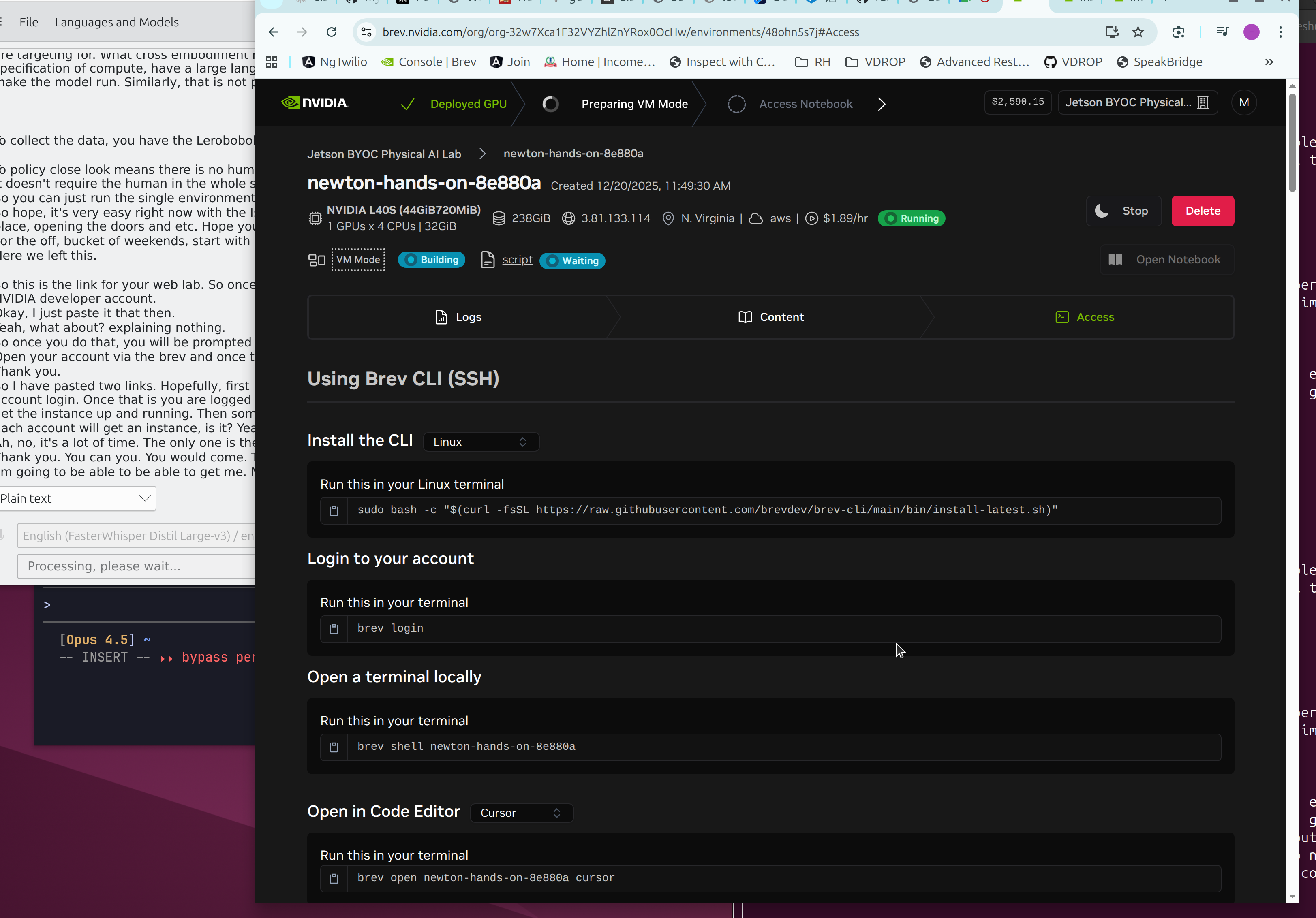
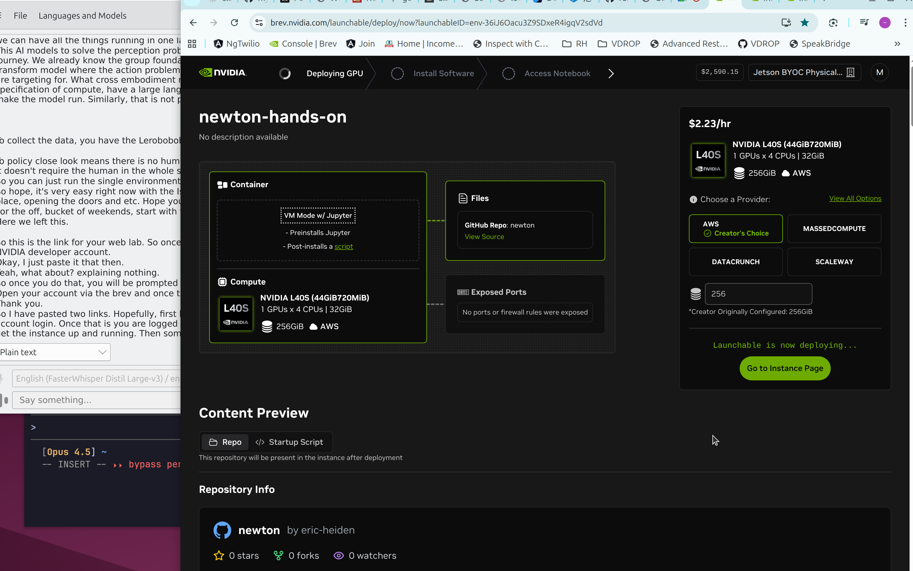
| Spec | Value |
|---|---|
| GPU | NVIDIA L40S (44GB VRAM) |
| Cost | $1.89/hour |
| Region | N. Virginia (AWS) |
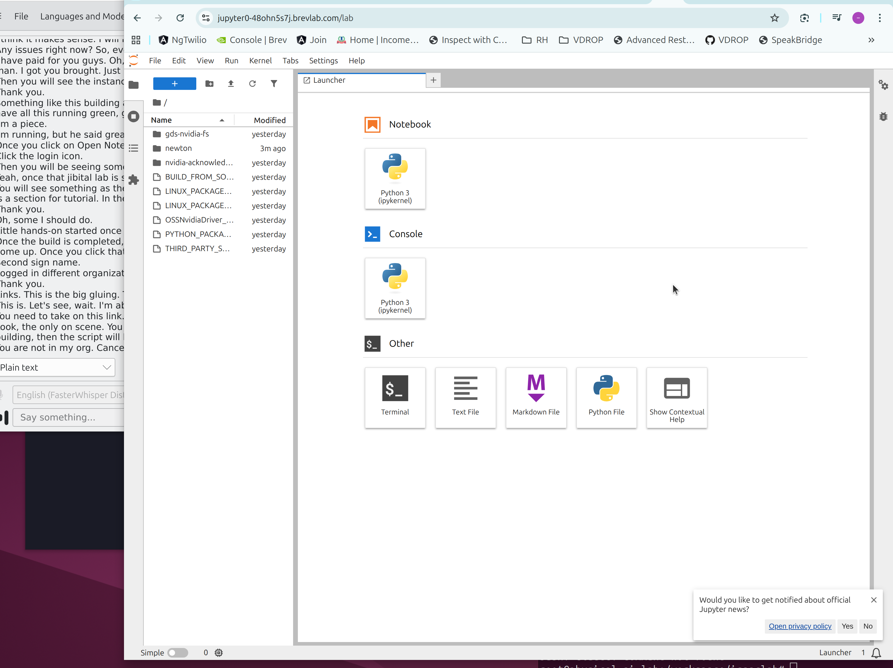
Tutorial Notebooks:
00_introduction.ipynb- Newton basics01_articulations.ipynb- Joint systems02_inverse_kinematics.ipynb- IK solving03_joint_control.ipynb- Control strategies04_domain_randomization.ipynb- Sim-to-real transfer05_robot_policy.ipynb- RL policy training06_diffsim.ipynb- Differentiable simulation
Simulation Results
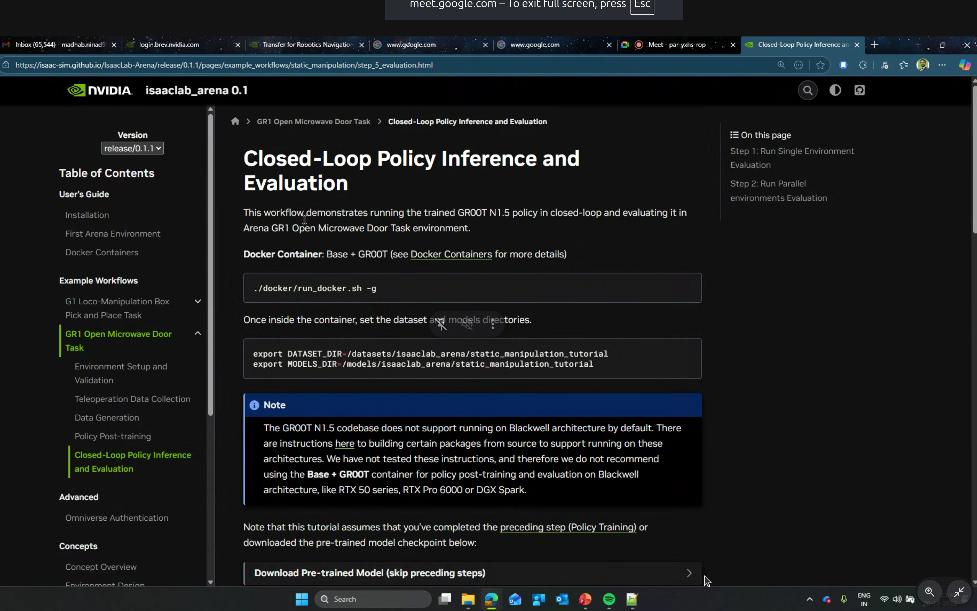
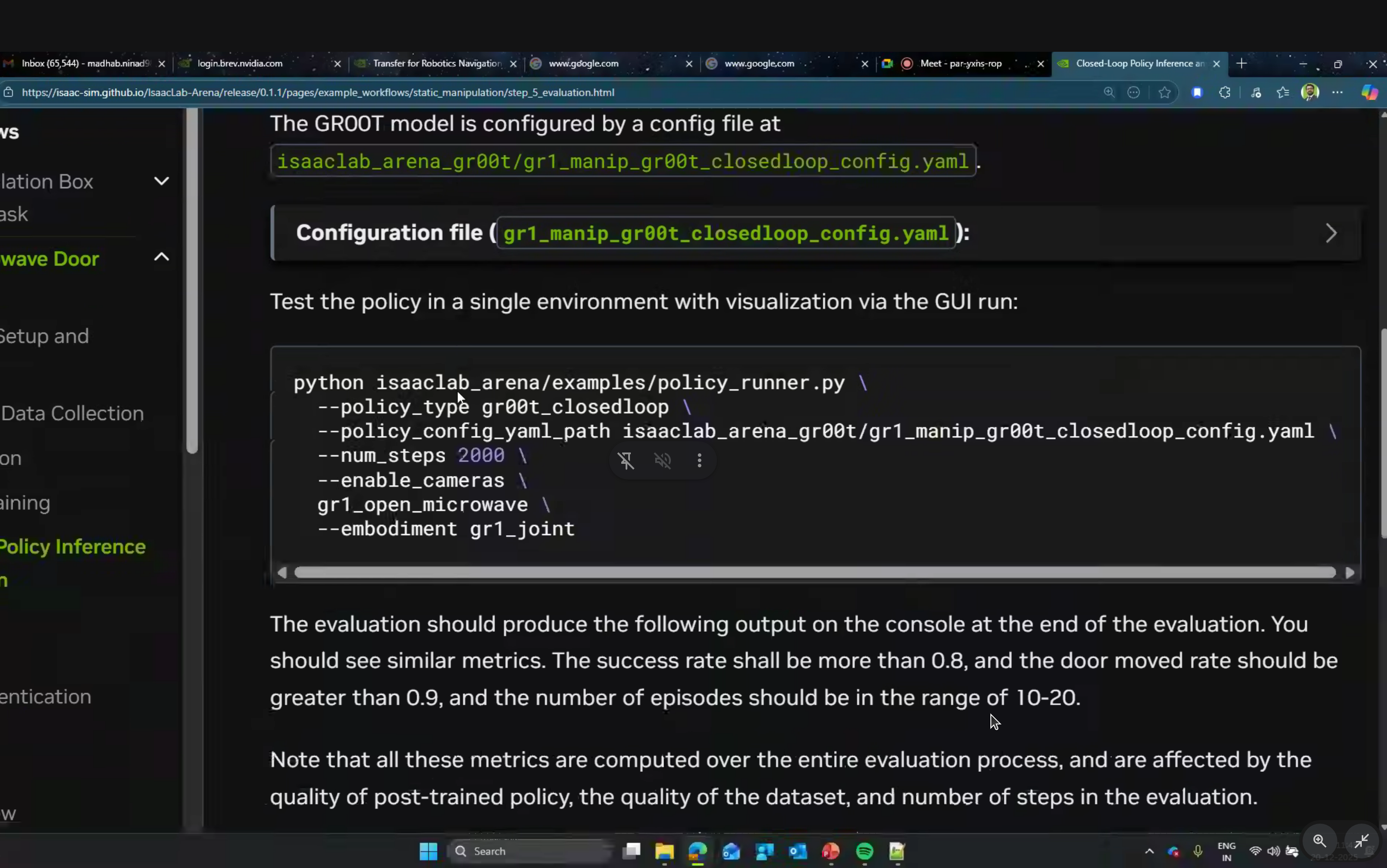
The GROOT N1.5 codebase does not yet support running on Blackwell architecture (RTX 50 series, RTX Pro 6000, DGX Spark). Use the Base + GROOT container for policy post-training and evaluation on Blackwell GPUs.
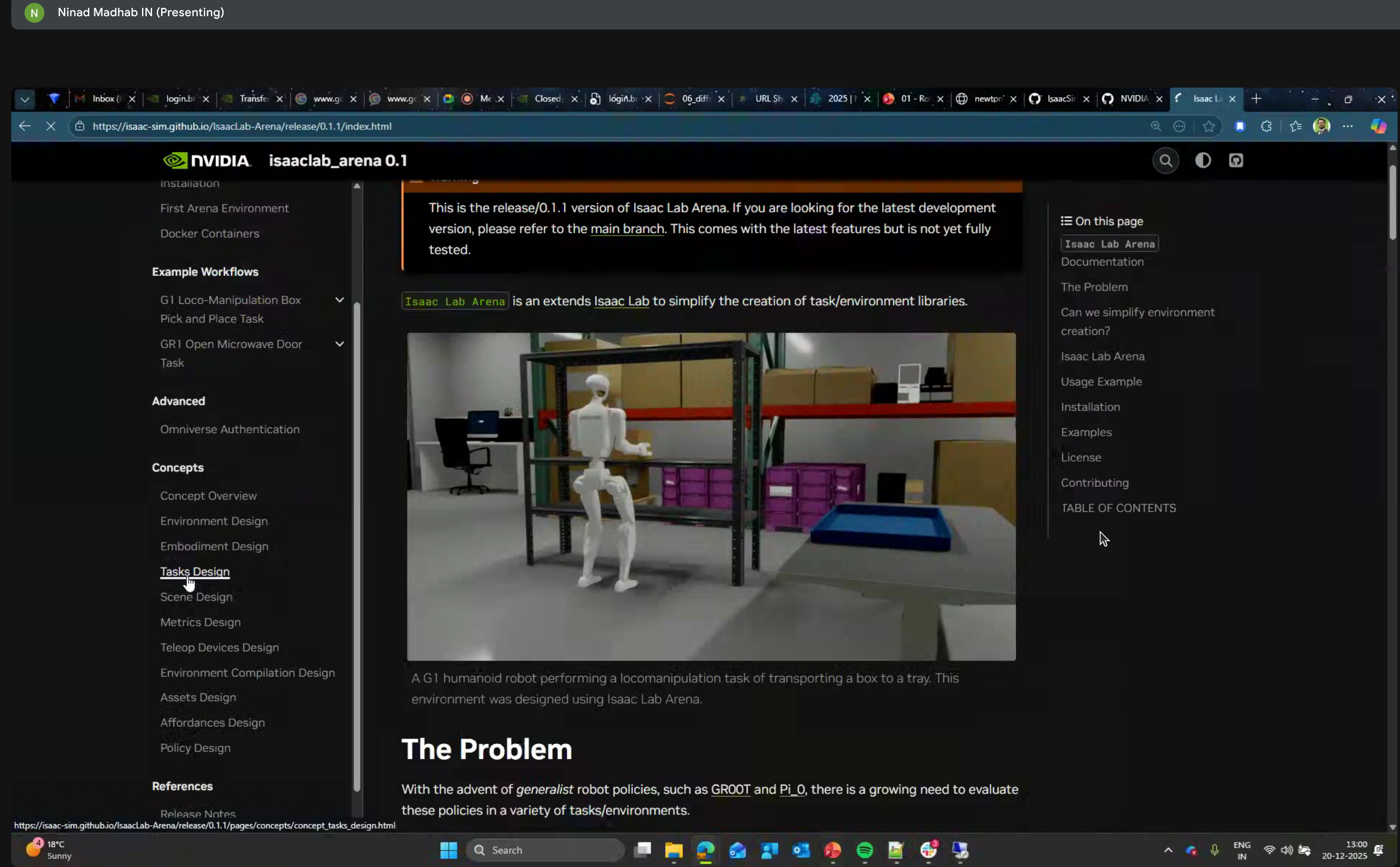
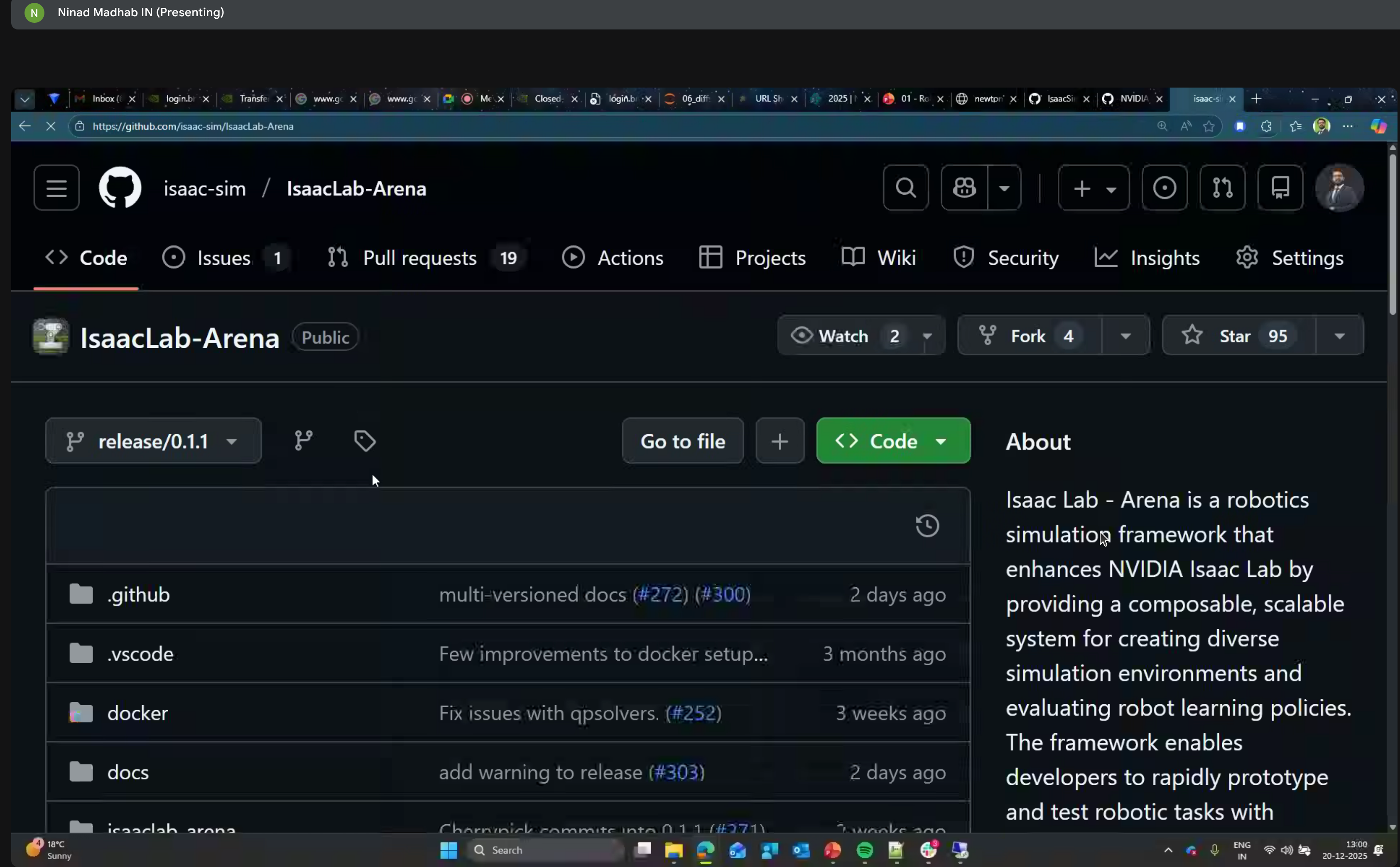
Isaac Lab Arena
For policy evaluation, NVIDIA provides Isaac Lab Arena - a framework for closed-loop policy inference:
Tasks Design
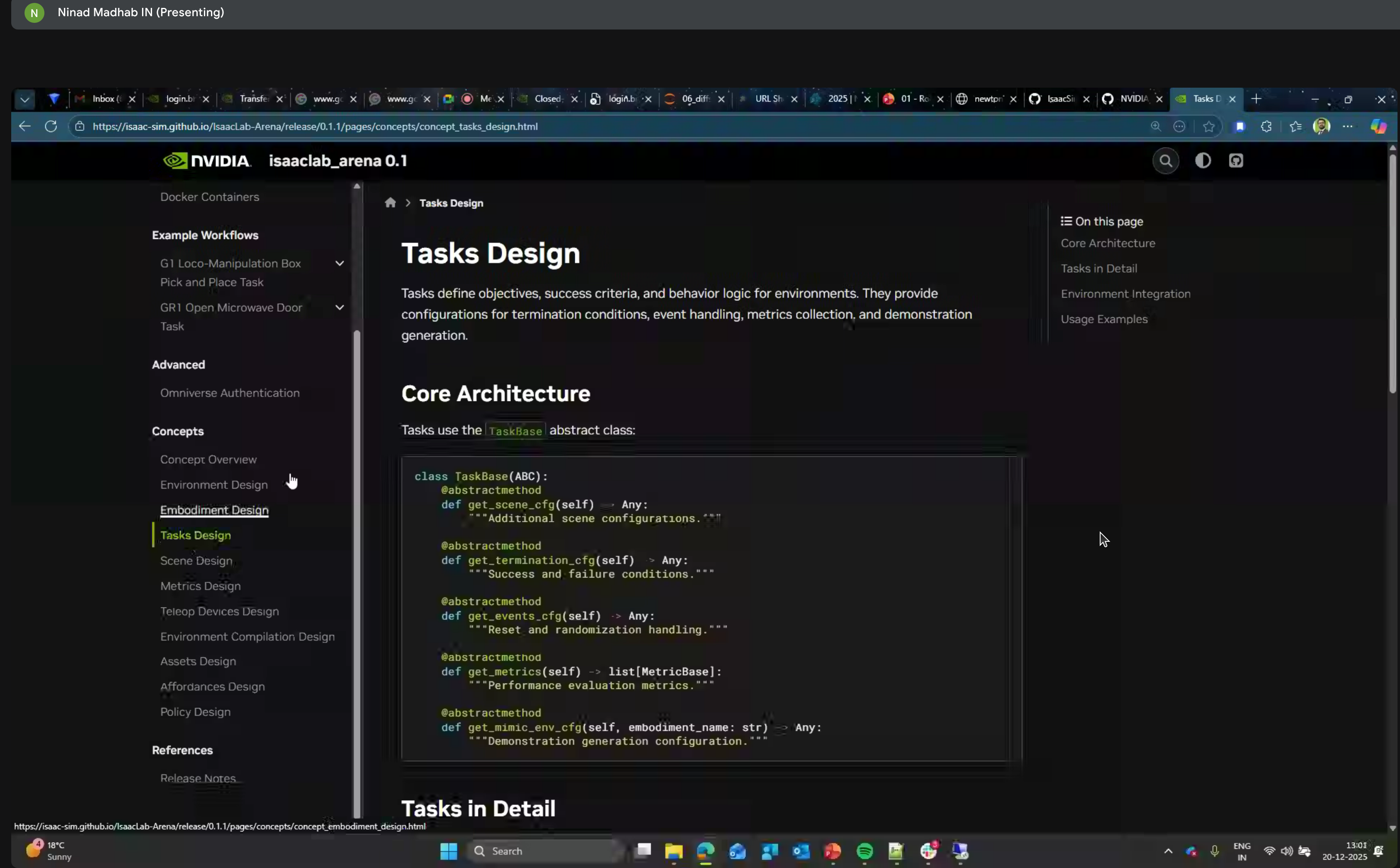
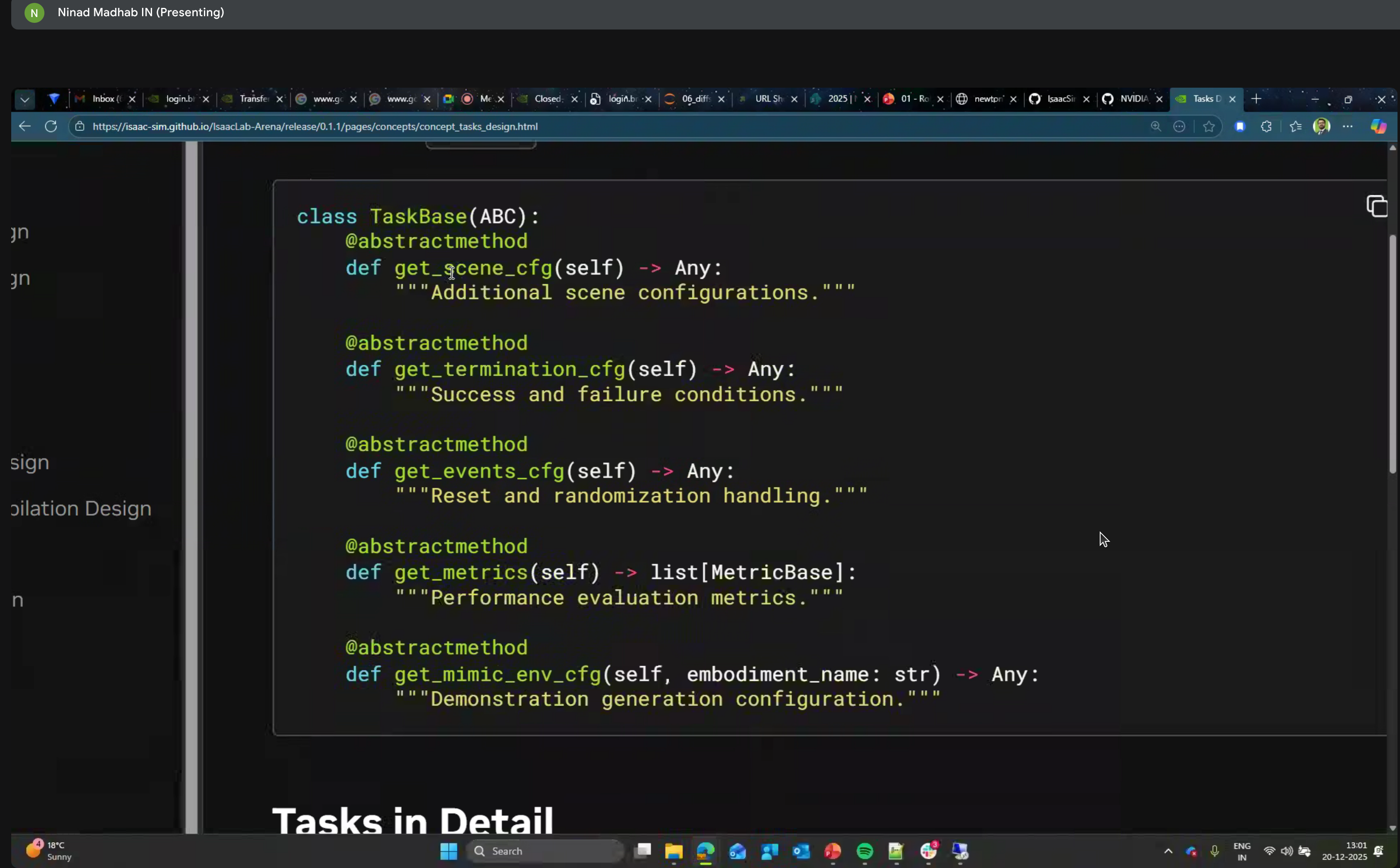
Tasks are defined using the TaskBase abstract class:
class TaskBase(ABC):
    @abstractmethod
    def get_scene_cfg(self) -> Any:
        """Additional scene configurations."""

    @abstractmethod
    def get_termination_cfg(self) -> Any:
        """Success and failure conditions."""

    @abstractmethod
    def get_events_cfg(self) -> Any:
        """Reset and randomization handling."""

    @abstractmethod
    def get_metrics(self) -> list[MetricBase]:
        """Performance evaluation metrics."""

    @abstractmethod
    def get_mimic_env_cfg(self, embodiment_name: str) -> Any:
        """Demonstration generation configuration."""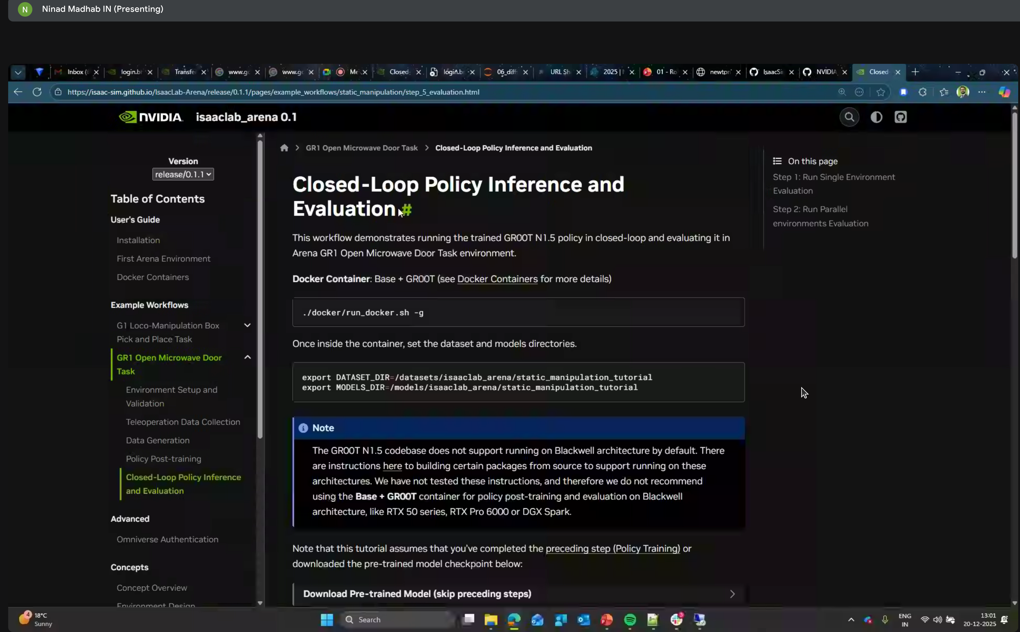
Example workflows include:
- G1 Loco-Manipulation Box
- Pick and Place Task
- GR1 Open Microwave Door Task
ROS Integration
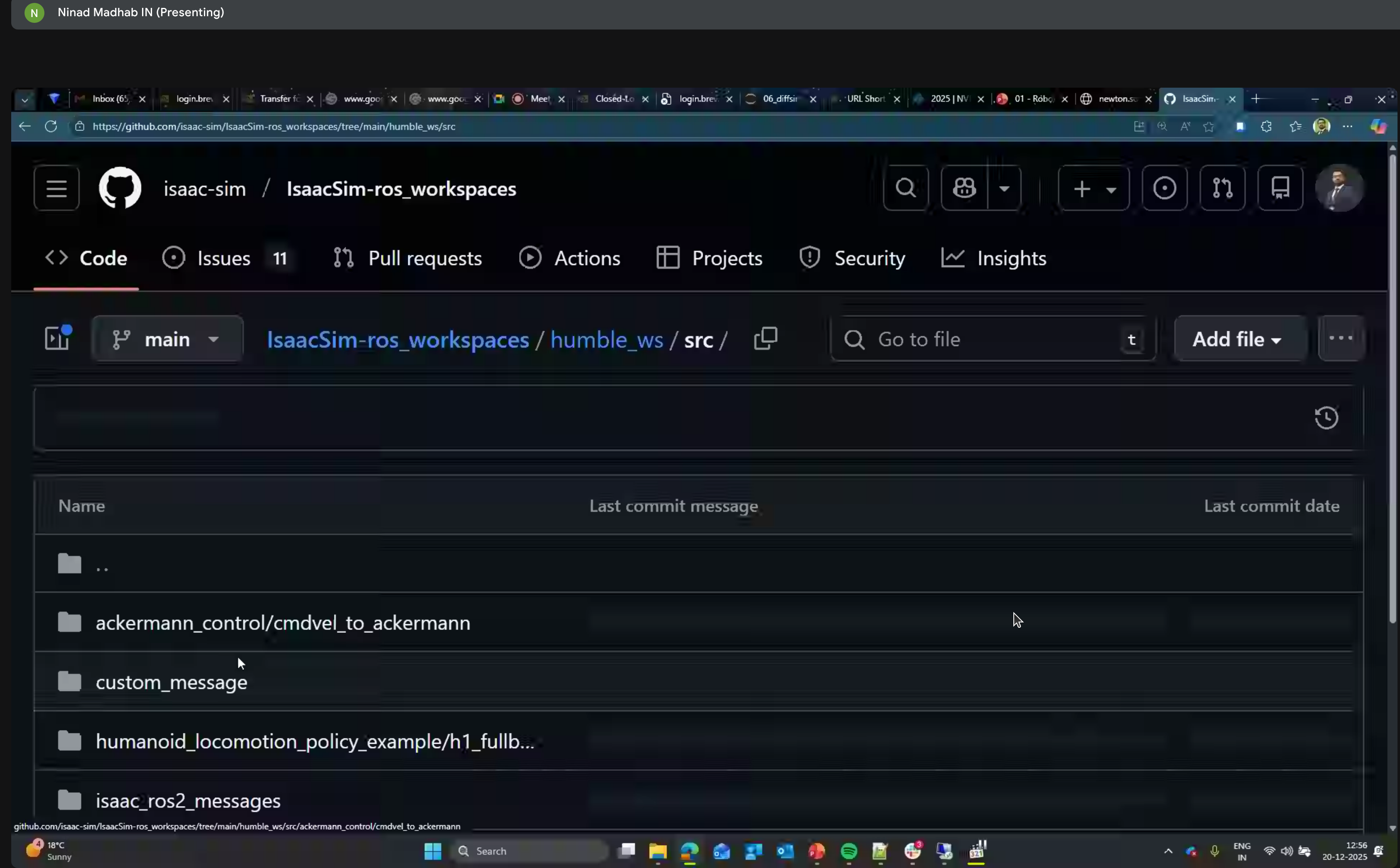
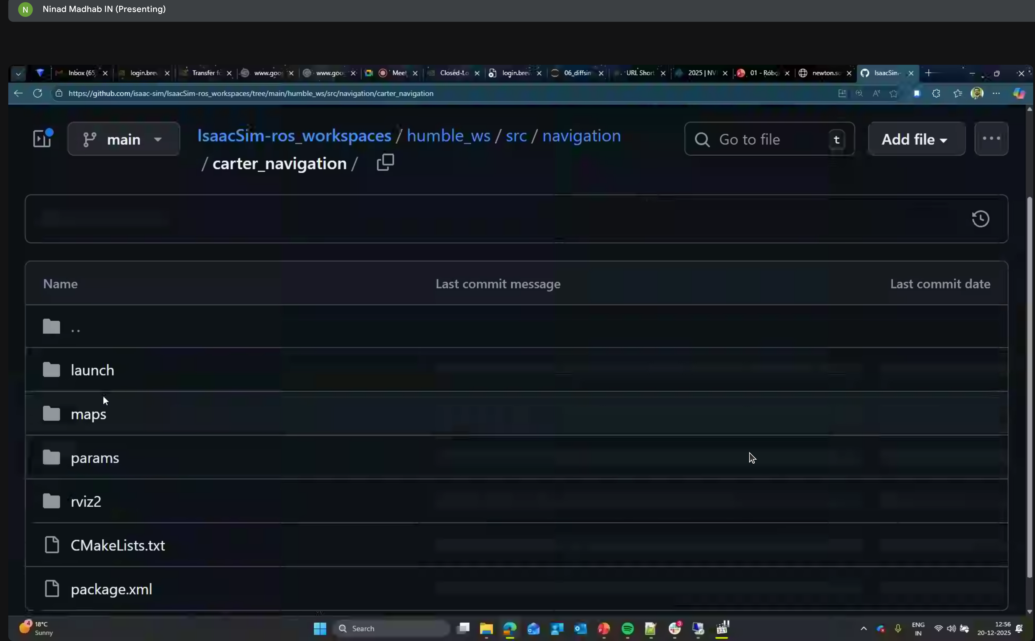
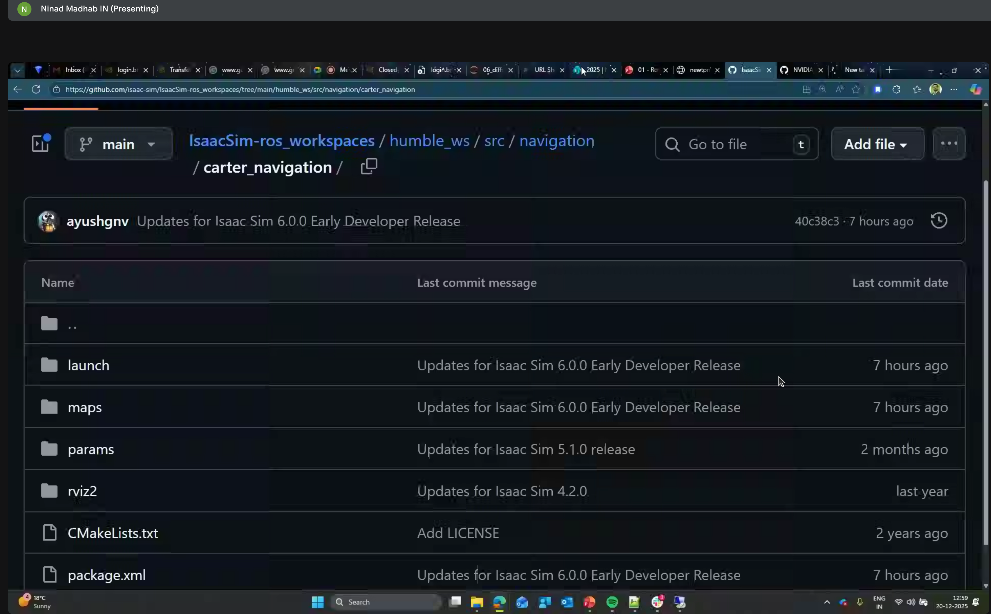
ROS2 NanoLLM
ROS2 nodes for LLM, VLM, and VLA using NanoLLM optimized for NVIDIA Jetson Orin.
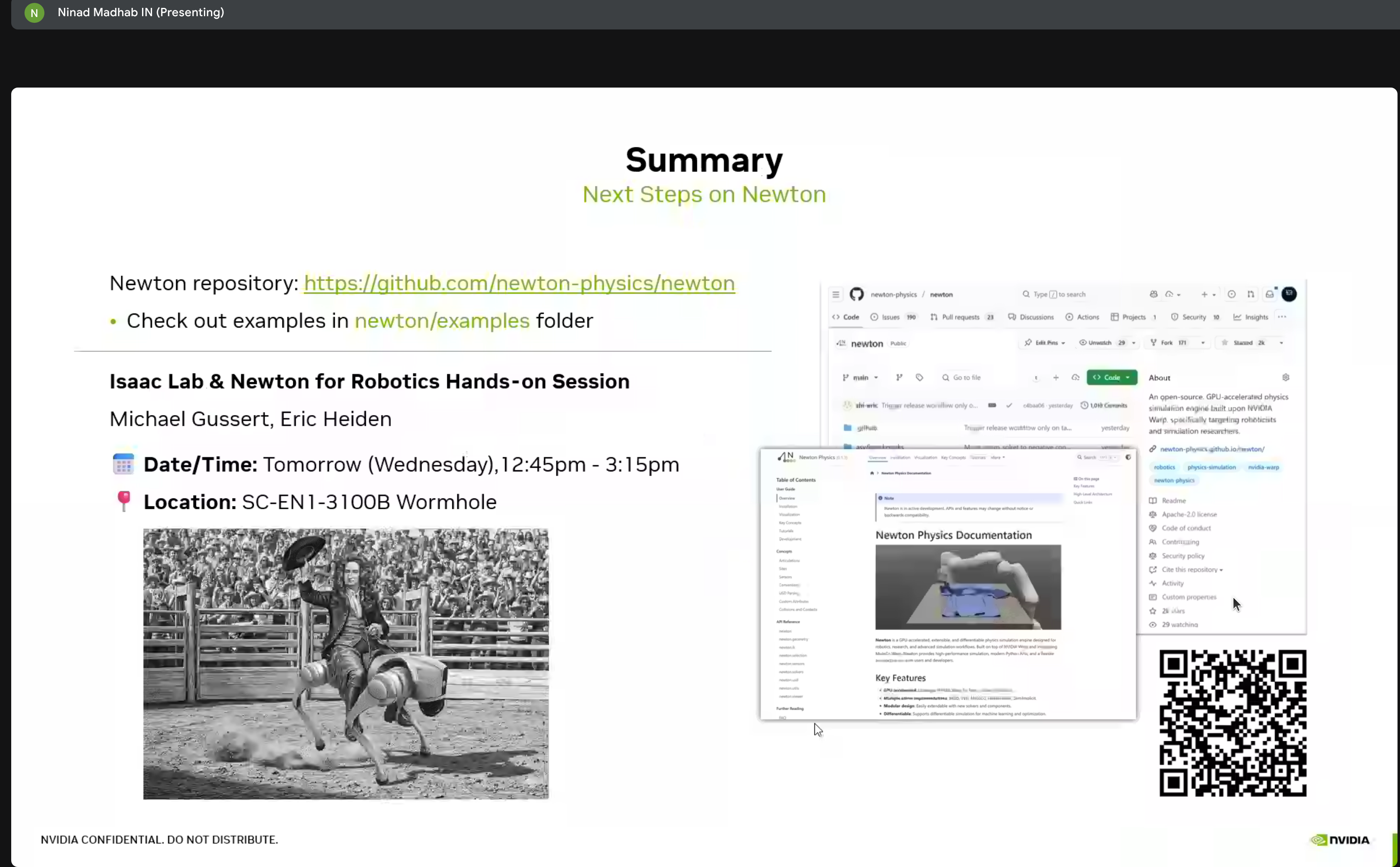
Newton Repository
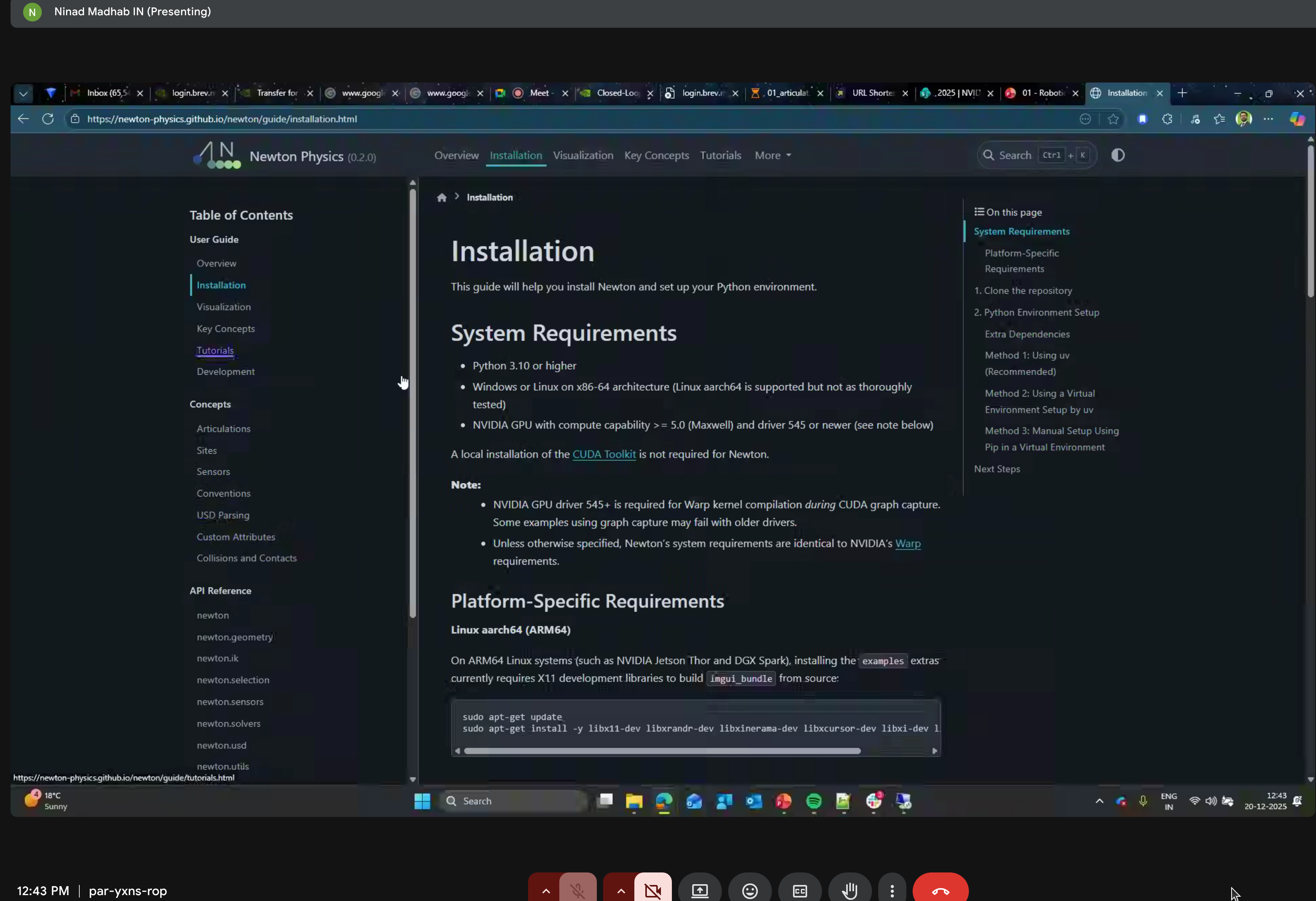
System Requirements
- Python 3.10+
- NVIDIA GPU compute capability 5.0+
- Platform-specific requirements for ARM64
Summary & Next Steps
Key Takeaways
Newton is production-ready - Open source, backed by major players, actively developed
MuJoCo integration - Newton can use MuJoCo as a solver backend, bringing the best of both worlds
Differentiable by design - Every component supports gradient computation for end-to-end learning
USD-native - Deep integration with Universal Scene Description for Omniverse compatibility
Scaling is the key - The GROOT-Mimic pipeline shows how to go from 10 demos to 1M training examples
Next Steps
Based on this workshop, I plan to:
- Try Newton locally - Install and run the tutorial notebooks on my RTX 5090
- Integrate with Isaac Lab - Use Newton as an alternative physics backend
- Explore GROOT-Mimic - Test the demonstration multiplication pipeline
- Build custom environments - Create Newton-based tasks for Go2-W training
Community Resources
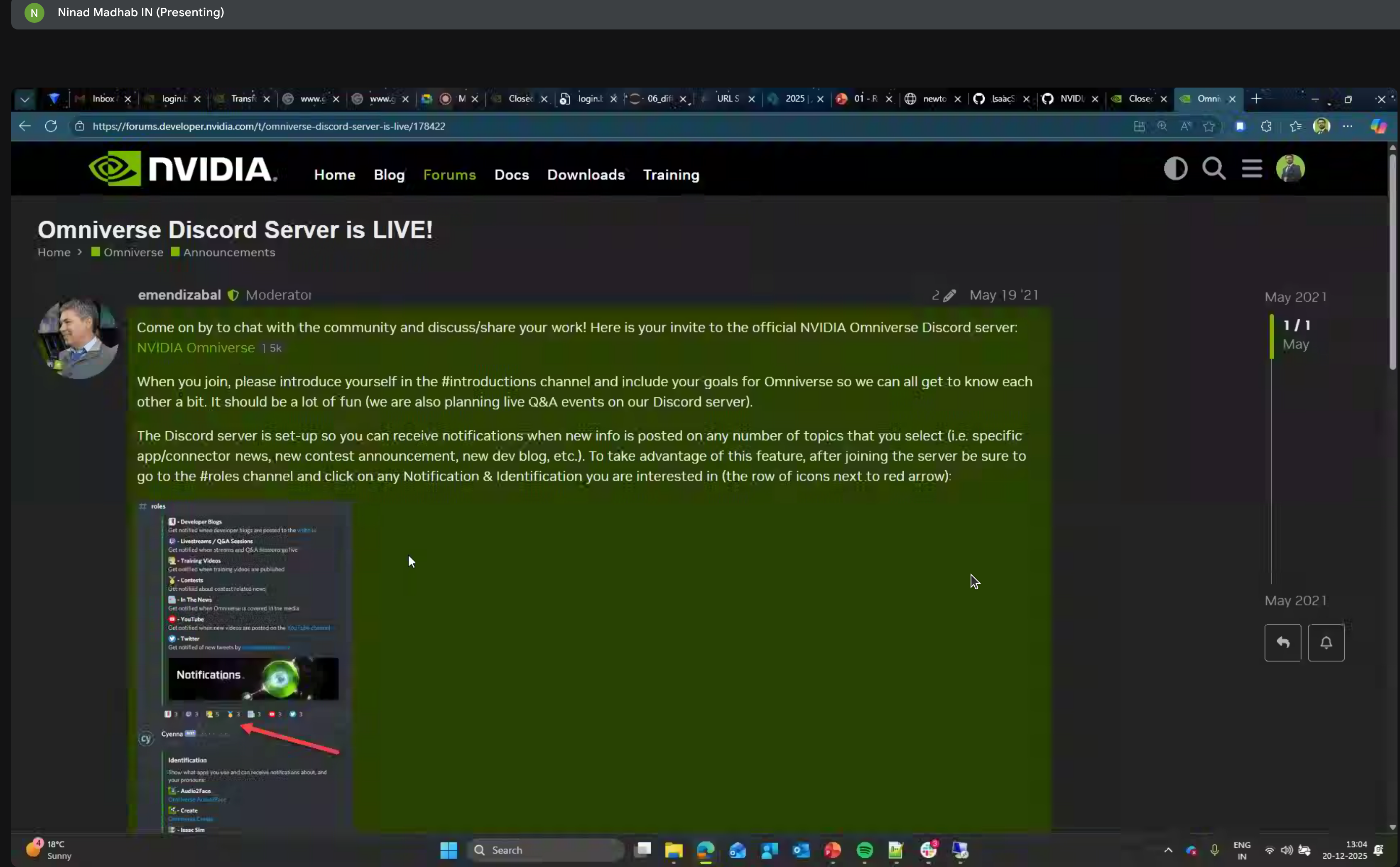
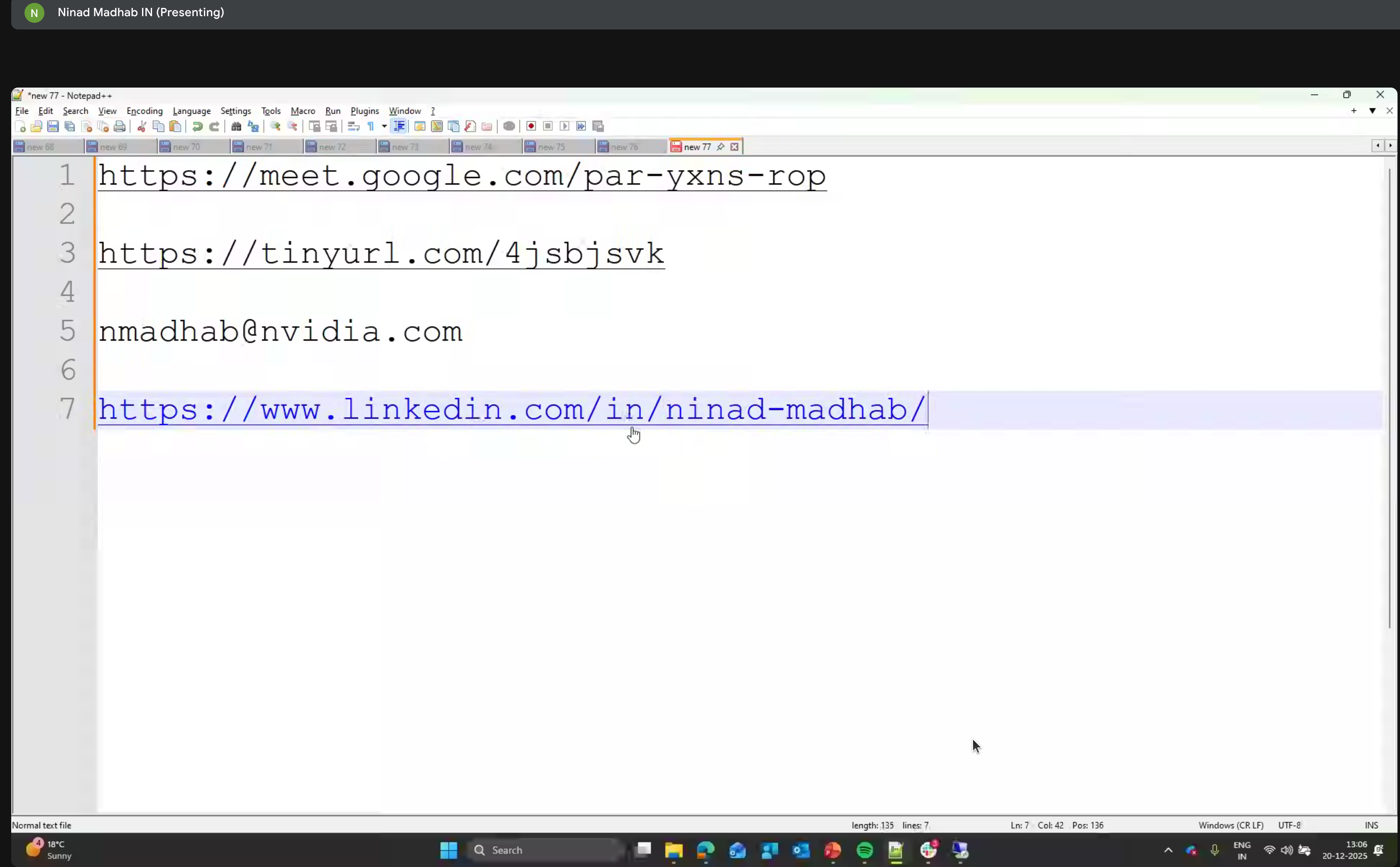
Resources
- Newton GitHub Repository (Apache 2.0)
- NVIDIA Warp - The underlying GPU compute framework
- Isaac Lab Arena Documentation
- Brev.dev - Cloud GPU platform for hands-on labs
This workshop was part of NVIDIA’s ongoing Physical AI education series. The combination of Cosmos, Newton, and Isaac Lab represents a comprehensive stack for developing embodied AI agents.