Lesson 4: ACT - Action Chunking with Transformers
The Architecture That Made Imitation Learning Work
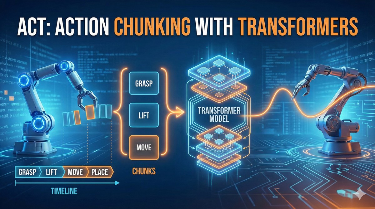
In this lesson, we decode ACT (Action Chunking with Transformers) - the policy that proved imitation learning can work on low-cost hardware. By the end, you’ll understand how VAEs and Transformers combine to make robots move smoothly.
🎧 Prefer to listen? Experience this lesson as an immersive classroom audio.
Chapter 1: The Promise of Low-Cost Robotics
Dr. Nova, I’ve been thinking about something. In Lesson 2, we learned about VAEs - how they compress data into latent variables. In Lesson 3, we mastered transformers - attention, encoders, decoders. But you kept promising we’d see how these pieces fit together in a real robot policy. I’m ready!
leans forward with excitement
Perfect timing. Today we’re going to decode one of the most influential papers in modern robot learning - ACT: Action Chunking with Transformers. This paper came out in 2023 and it fundamentally changed what people thought was possible with imitation learning.
But before I show you the architecture, let me ask you something. How much do you think a capable research robot setup costs?
Based on what I’ve heard… probably hundreds of thousands of dollars? Industrial robot arms, specialized sensors, custom grippers…
That’s exactly what everyone assumed! Before 2023, if you wanted to do serious manipulation research - the kind where robots learn complex tasks - you needed budgets in the hundreds of thousands of dollars. Labs at Stanford, Berkeley, Google… they had the resources. Small research groups? Students who wanted to experiment? Locked out.
Then the ACT paper dropped a bombshell.
What kind of bombshell?
Twenty thousand dollars.
That’s the total budget for the entire ALOHA system - four robot arms, multiple cameras, the whole setup. And it wasn’t some toy demo. It achieved tasks that $100,000+ systems couldn’t reliably do.
Wait, ALOHA? Like the Hawaiian greeting?
chuckles
It’s an acronym: A Low-cost Open-source Hardware system for bimanual teleoperation. The name is playful, but the impact was serious. Let me show you the setup.
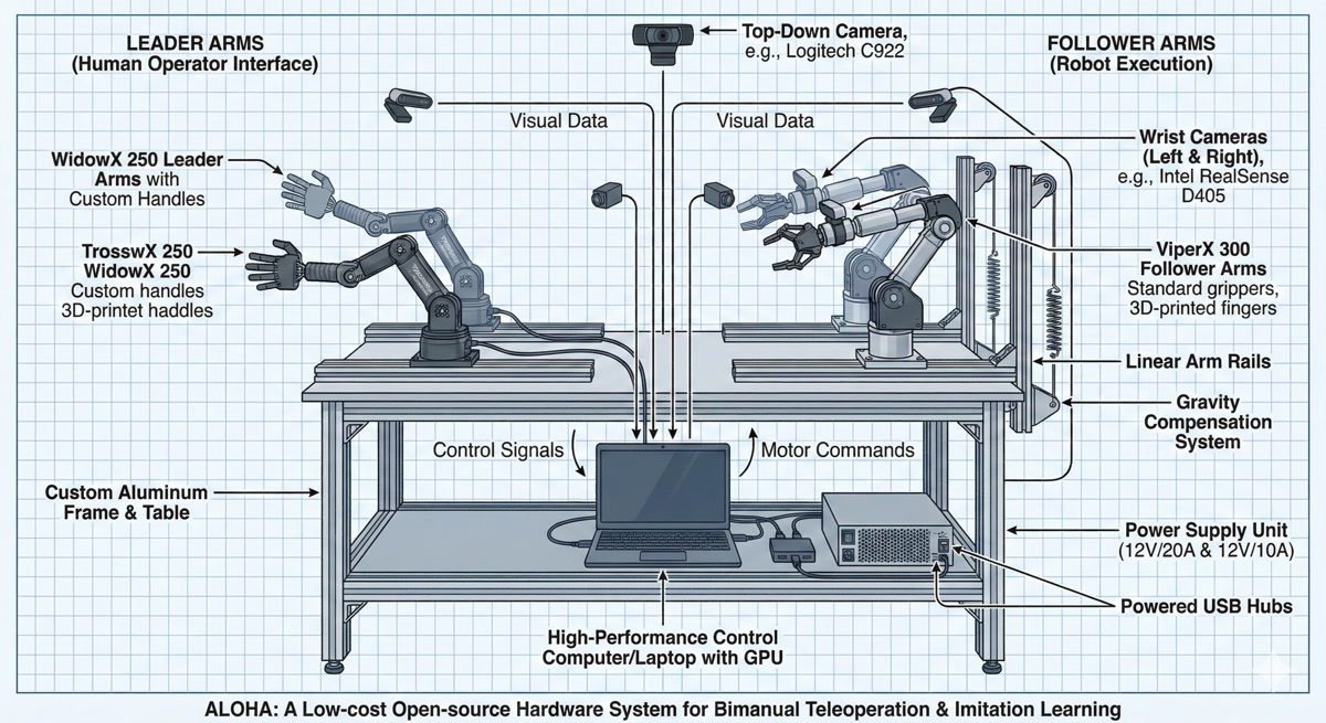
See how there are four arms? That’s the key to bimanual manipulation - tasks that require two hands working together.
Like our SO-ARM101 setup! We have two Leader arms and two Follower arms too.
Exactly! Your setup follows the same philosophy. The ALOHA paper proved that this Leader-Follower architecture could work for real research. Here’s the breakdown:
| Component | Purpose | Cost |
|---|---|---|
| 4 Robot Arms | 2 Leaders + 2 Followers | ~$13,200 |
| 4 Cameras | Top, front, 2 wrist-mounted | ~$400 |
| 3D Printed Parts | Mounts, grippers | ~$500 |
| Computer + Misc | Processing, cables, table | ~$6,000 |
| Total | ~$20,000 |
Now, $20,000 might still sound like a lot compared to your SO-ARM101 kit. But remember - research labs were spending 5-10x this for systems that performed worse.
You said it performed tasks that expensive systems couldn’t do. What kind of tasks?
pulls up demonstration videos
This is where it gets exciting. Let me show you three tasks that made the robotics community pay attention:
Task 1: Opening a Ziplock Bag
Think about what’s involved here. One arm holds the bag, the other finds and grips the tiny seal, then pulls with just the right force - not too hard (rips the bag) or too soft (doesn’t open). This requires incredibly fine-grained coordination.
Task 2: Inserting a Battery
One arm holds a remote control steady, the other picks up a battery and slots it in - with the correct orientation. Miss the slot by a few millimeters and you fail.
Task 3: Opening a Cup Lid
Sounds simple, right? But the lid might be on tight. The cup might slip. Both arms need to work together, adjusting grip pressure in real-time.
These all require both hands working together. That’s why it’s called bimanual manipulation.
Precisely! And here’s the stunning result - the comparison against other methods:
| Task | ACT | Other Methods |
|---|---|---|
| Ziplock Opening | 84% | 0-12% |
| Battery Insertion | 96% | 0-8% |
Most other methods completely failed on these tasks - literally 0% success rate. ACT wasn’t just better, it was in a different league entirely.
One of the co-authors is Sergey Levine, a pioneer in robot learning who later co-founded Physical Intelligence - a company building general-purpose robot policies. When researchers at this level are publishing, you know the ideas are solid.
sits back, processing
So we have accessible hardware… impressive results… but there must be a secret sauce in the software, right? What makes ACT different from all those methods that scored zero?
smiles knowingly
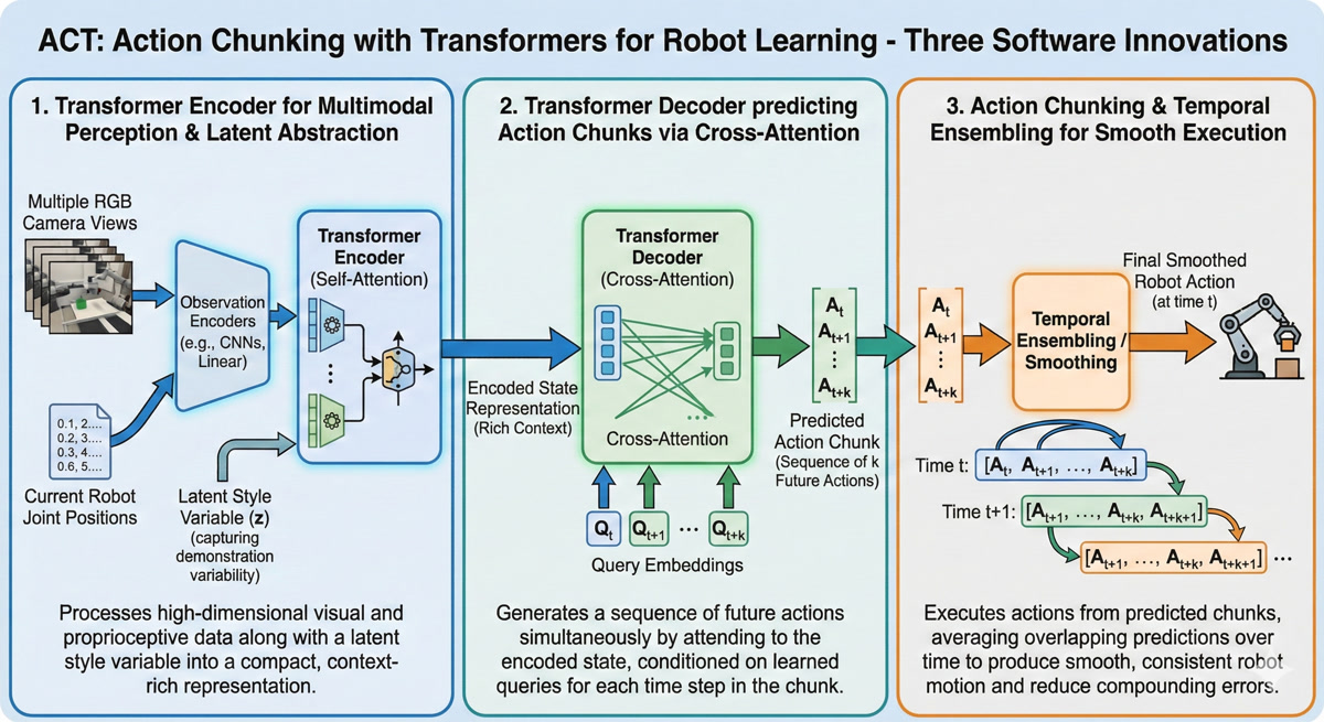
Now you’re asking the right question. The hardware democratized access, but the real innovation is in the software. ACT combines three key ideas - and two of them you already understand from our previous lessons!
| Innovation | What You Already Know | What’s New |
|---|---|---|
| Conditional VAE | Lesson 2: Encoder → Z → Decoder | Applied to robot actions |
| Transformer Decoder | Lesson 3: Cross-attention, Q/K/V | DETR-inspired parallel prediction |
| Action Chunking | New concept! | Predicting K actions at once |
The CVAE captures the style of how to do a task. The transformer decoder fuses information from multiple cameras. And action chunking ensures the robot moves smoothly, not jerkily.
I remember in Lesson 2, we talked about the multimodal problem - how averaging two good solutions gives you a bad solution. Does the CVAE solve that here too?
eyes light up
That’s exactly where we’re headed! But I’m not going to show you the complete architecture right away. That would be like showing you the assembled puzzle before you understand why each piece exists.
Instead, we’re going to build ACT from first principles - piece by piece. By the time we reach the full architecture, you won’t just recognize it… you’ll understand it.
Let me ask you this: if someone shows you a cup-picking demonstration ten times, and each time they take a slightly different path to the cup… how should the robot decide which path to take?
pauses
I… want to say “average them”? But from Lesson 2, I know that’s wrong. Averaging different paths could send you straight into an obstacle…
You’re on the edge of the key insight. Hold that thought - we’ll resolve it in Chapter 3 when we dive into the CVAE encoder. For now, just know that ACT has a clever answer to this problem.
Ready to see how it all connects to what we’ve learned?
Absolutely. I feel like everything from Lessons 2 and 3 is about to click into place.
That’s exactly what’s about to happen. Let’s go!
Chapter 2: Building on Foundations
Okay, I’m excited about the hardware being accessible. But you mentioned three software innovations - CVAE, Transformer Decoder, and Action Chunking. Can we dig into what makes this combination special?
Absolutely. And here’s what I love about ACT - it’s not magic. It’s built on concepts you already understand from our previous lessons. Let me show you how.
Each innovation addresses a specific challenge:
studying the interactive guide
So the CVAE handles… the variety in demonstrations? Like different styles?
nods approvingly
Exactly right! Let’s break down what each innovation does:
Innovation 1: Conditional VAE (CVAE)
Remember in Lesson 2 when we talked about the multimodal problem? You can’t just average different expert demonstrations because you get something that’s worse than any of them.
The CVAE captures the style of a demonstration. When ten people show you how to pick up a cup, they all do it slightly differently - some go from the left, some from the right, some lift higher. The CVAE learns to encode these different styles into a latent variable Z.
So Z is like… a “style selector”? It doesn’t average the styles, it picks one?
eyes light up
You’re already seeing it! That’s the key insight we’ll explore deeply in Chapter 3. For now, just know that Z lets the model commit to ONE coherent trajectory instead of some blurry average.
Innovation 2: Transformer Decoder (DETR-inspired)
This is where Lesson 3 pays off. Remember cross-attention? How the decoder can query the encoder to get relevant information?
ACT uses a transformer encoder to fuse information from multiple cameras - top view, front view, wrist cameras. All those different perspectives get combined into a rich representation. Then the decoder uses cross-attention to extract exactly what it needs to predict actions.
Wait - so it’s not just “one camera, one prediction”? It’s fusing multiple viewpoints?
Precisely! And this is crucial for bimanual manipulation. When you’re opening a ziplock bag, the top camera sees the overall scene, but the wrist cameras see the fine details of where your fingers are gripping. You need ALL of that information fused together.
The transformer encoder inside the decoder takes 1202 tokens - we’ll break down exactly where that number comes from in Chapter 5 - and creates a unified understanding of the scene.
Innovation 3: Action Chunking
This one is new - we didn’t cover it in previous lessons. Here’s the problem: if you predict one action at a time, small errors compound.
Compound? Like… the error grows?
draws in the air
Imagine you’re trying to draw a straight line, but after each millimeter, someone nudges your hand slightly. By the time you’ve drawn ten centimeters, you’re way off course!
That’s what happens with single-action prediction. Each prediction has a tiny error. The robot acts on that prediction. Now it’s in a slightly wrong position. The next prediction is based on that wrong position, adding more error. It drifts.
Action chunking solves this by predicting K actions all at once - typically K=100. Instead of “what’s my next action?”, the model asks “what are my next 100 actions?”. The robot executes a chunk, then gets a fresh prediction, resetting any accumulated error.
connecting the dots
So it’s like… course correction? You drift a little during a chunk, but then you get a new, accurate chunk that puts you back on track?
Exactly! And there’s another benefit - smoothness. When you predict one action at a time at high frequency, even small inconsistencies make the robot jittery. But a chunk of 100 actions is predicted all at once, ensuring they’re internally consistent. The motion is smooth.
Let me ask you something: why do you think we need to predict distributions of actions rather than just single actions?
thinks back to Lesson 2
Because… because of the multimodal problem! If the training data has multiple valid ways to do something, and we try to predict a single “best” action, we might average them and get something invalid.
beaming
Perfect callback! This is exactly why the CVAE is essential. Let me give you a concrete example:
Imagine teaching your SO-ARM101 to pick up a block. In 50 demonstrations, you approached from the left. In 50 others, you approached from the right. Both are perfectly valid!
Now, what happens if we train a simple neural network to predict the “average” action?
realizes with horror
It would predict an action that goes… straight down the middle? Which might hit the block from above and knock it over!
snaps fingers
Exactly! The average of two good solutions is often a terrible solution. This is why ACT uses a CVAE:
| Approach | What It Does | Problem |
|---|---|---|
| Single prediction | Outputs one action | Averages valid modes → invalid action |
| CVAE | Samples Z, then predicts action conditioned on Z | Commits to ONE mode → valid action |
The CVAE doesn’t average the left and right approaches. It samples a Z that commits to either left OR right, then predicts a coherent trajectory for that choice.
So the three innovations work together - CVAE handles multimodality, transformers fuse multi-camera information, and action chunking prevents drift and ensures smooth motion.
You’ve got it! And here’s the beautiful thing - none of these ideas are new in isolation:
- CVAEs existed since 2015
- Transformers revolutionized NLP in 2017
- Action chunking builds on temporal abstraction ideas from hierarchical RL
What ACT did was combine them in the right way for robot manipulation. The paper’s contribution isn’t inventing new components - it’s showing how to architect them together.
Ready to dive deep into the first innovation - the CVAE encoder that captures demonstration style?
Yes! I want to understand exactly how Z works. How does it “choose” a style instead of averaging?
That’s our next chapter - and it’s where the real “aha” moment happens. Let’s go!
Chapter 3: The CVAE Encoder
scratching head
Okay, I understand WHY we need to avoid averaging - the multimodal problem. But I still don’t get HOW the CVAE actually solves it. How does sampling a Z magically prevent averaging?
pauses thoughtfully
You know what? Instead of me explaining, let me show you what goes wrong WITHOUT the CVAE. Then you’ll see exactly why it’s essential.
Let’s simulate training your SO-ARM101 to pick up a block. You record 100 demonstrations - 50 where you approached from the left, 50 from the right.
Both valid ways to pick it up!
Exactly. Now, let’s train a simple neural network - no CVAE, just: image → MLP → predicted action.
During training, the network sees demonstrations from both sides. The loss function says “minimize the error between your prediction and the demonstrated action.”
What do you think the network learns to predict?
thinking
If it sees half the demos going left and half going right… it would try to minimize error for BOTH… so it would predict something in the middle?
draws on the whiteboard
Let’s see exactly what happens. The loss function for each training example is:
\[\text{Loss} = || \text{predicted action} - \text{demonstrated action} ||^2\]
The network wants to find ONE prediction that minimizes this across ALL examples. What’s the mathematical answer?
The mean! The average of all demonstrated actions!
snaps fingers
Exactly right. And when you average “approach from left” with “approach from right”…
eyes widen
You get “approach from straight ahead” - which hits the block from the top and knocks it over!
The average of two valid solutions is INVALID!
nods gravely
This is the fundamental problem. Traditional supervised learning optimizes for the EXPECTED action. But in robotics, the expected action is often catastrophic.
Now, here’s where the CVAE changes everything. Let me show you with an interactive visualization.
The CVAE doesn’t find the average style.
It samples ONE style and commits to it.
| Approach | What Happens | Result |
|---|---|---|
| No CVAE | Network predicts E[action] = average | Invalid trajectory (middle path) |
| With CVAE | Network samples Z, then predicts action | Z |
The magic is in the conditioning: action GIVEN Z, not just action.
slowly nodding
So Z is like… a switch? When Z = 0.5, predict the left trajectory. When Z = -0.5, predict the right trajectory. But never average them?
beaming
That’s the eureka moment! Z partitions the output space. Different regions of Z correspond to different valid trajectories. The network learns: “Given THIS value of Z, predict THIS coherent trajectory.”

Let me show you exactly how the encoder architecture captures this style information.
Wait - the encoder. In Lesson 2, our VAE encoder took images and produced Z. What does ACT’s encoder take as input?
This is a subtle but crucial design choice. ACT’s encoder sees joint angles and actions - NOT images.
confused
Why exclude images? Don’t they contain important information?
pulls up a diagram
Think about it: two humans might see the exact same cup in the exact same position, but one reaches from the left and one from the right. The visual input is identical - the difference is purely in their style of movement.
Style lives in the trajectory, not in what the robot sees.
| Component | Input | What It Learns |
|---|---|---|
| Encoder | Joints + Actions | “How does this person move?” (style Z) |
| Decoder | Images + Joints + Z | “What should I do now?” (predicted actions) |
The encoder learns how humans move differently. The decoder uses that + current observation to decide what to do.
In Lesson 2, our VAE encoder was just an MLP. But robot actions come in sequences - Action 1 affects Action 2 affects Action 3…
eyes light up
Exactly! And what did we learn in Lesson 3 captures relationships in sequences?
Transformers! The self-attention mechanism finds relationships between different positions in a sequence!
beams
So ACT uses a transformer encoder instead of an MLP. Here’s the architecture:
INPUT TO ENCODER:
├── Current joint angles (6 values for 6-DOF arm)
├── Action chunk (K future actions, each with 6 values)
└── CLS token (learnable summary token)
Everything gets tokenized and embedded. The joint angles become one token. Each action becomes one token. And we add a special CLS token - remember that from Vision Transformers?
The CLS token attends to everything else and becomes a summary of the whole sequence!
Exactly! Let me draw what happens inside:
ENCODER ARCHITECTURE:

  [CLS]  [Joints]  [A₁]  [A₂]  [A₃]  ...  [Aₖ]
    │       │       │     │     │         │
    └───────┴───────┴─────┴─────┴─────────┘
                    │
             ┌──────▼──────┐
             │ + Position  │  (Add positional embeddings)
             │  Embedding  │
             └──────┬──────┘
                    │
             ┌──────▼──────┐
             │    Self     │  (Each token attends to all)
             │  Attention  │
             └──────┬──────┘
                    │
             ┌──────▼──────┐
             │    FFN      │  (Feed-forward network)
             └──────┬──────┘
                    │
    [ctx₀] [ctx₁] [ctx₂] [ctx₃] [ctx₄] ... [ctxₖ₊₁]
      │
      │  (Only CLS context used)
      ▼
   ┌──────────────────────────────────┐
   │  Project to μ and σ → Sample Z  │
└──────────────────────────────────┘So self-attention lets each action token “see” all other actions - Action 1 relates to Action 2, relates to Action 3…
Exactly! The CLS token attends to everything - joints and all K actions. Its final context vector holds a summary of the entire movement pattern.
This summary is projected to mean (μ) and variance (σ), then we sample Z using the reparameterization trick from Lesson 2.
Z encodes the hidden factors that differentiate how humans perform the same task:
| Z Value | Encoded Style |
|---|---|
| Z ≈ 0.5 | Wide arc reaching motion |
| Z ≈ -0.5 | Direct linear approach |
| Z ≈ 1.2 | Slow, cautious movement |
| Z ≈ -1.2 | Fast, confident movement |
During training, the encoder learns to map different demonstration styles to different regions of Z-space.
This is like the handwriting example from Lesson 2! Different people write “hello” with different slants and neatness - those hidden factors got encoded in Z.
Perfect analogy! And there’s strong evidence this design matters. The ACT paper includes an ablation study - they tested what happens when you remove the CVAE.
For the bimanual insertion task:
| Configuration | Success Rate |
|---|---|
| With CVAE | 90% |
| Without CVAE | 57% (-33 points!) |
Without the style variable, you’re back to averaging - and averaging valid solutions often produces invalid ones.
mind blown
So the encoder isn’t just nice to have - it’s essential. The 33-point drop proves that capturing style with Z is what makes ACT work!
Exactly. The CVAE encoder is the foundation that makes everything else possible.
Now, here’s a question for you: we’ve talked about Z capturing style during training, when we can see the future actions. But at inference time, when the robot is actually operating, we don’t know the future actions yet. So how do we get Z?
pauses
Hmm… we can’t use the encoder because it needs the action sequence as input… so we can’t sample from the learned distribution…
grins
This is where the “conditional” in CVAE becomes important. During inference, we sample Z from a prior distribution - typically a standard normal N(0,1). The decoder is trained to work with Z samples from both the encoder (during training) and the prior (during inference).
But we’re getting ahead of ourselves - that’s decoder territory. Ready to see how Action Chunking prevents the jerky, drifting motion problem?
Yes! I want to understand why K=100 actions instead of just 1.
Chapter 4: Action Chunking
Explore the key insight behind Action Chunking: “You don’t need perfect predictions. You need fewer opportunities to make mistakes.”
Navigate through 5 sections using the Next/Previous buttons. Drag to rotate the 3D view, scroll to zoom. Hover over objects for tooltips.
Great question about K=100. This is the Action Chunking innovation - and I’d argue it’s the most impactful contribution of the entire paper.
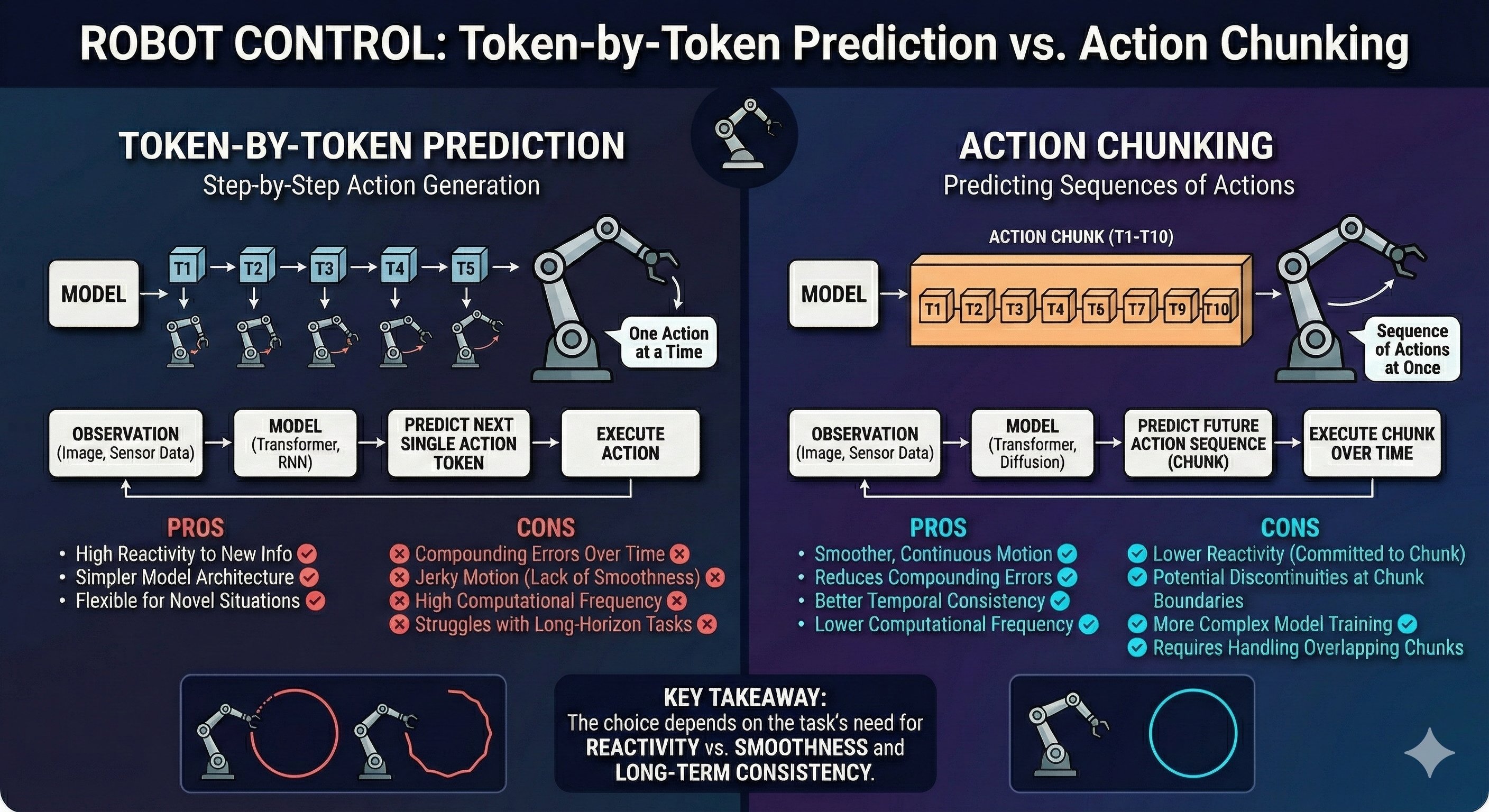
Let me start with a question: in LLMs like GPT, how does text generation work?
Token by token! The model predicts the next token, adds it to the sequence, then predicts the next one based on everything so far.
Exactly - autoregressive generation. Now, what if we applied the same approach to robotics? Predict one action, execute it, observe the new state, predict the next action…
That seems natural! It worked for language, why not robotics?
holds up a finger
Here’s the catch: there’s a critical problem in robotics that doesn’t exist - at least not as severely - in language.
Compounding errors.
Every prediction has a small error. In language, if you predict “the” instead of “a”, the sentence still works.
But in robotics, each error shifts the robot’s physical state:
TOKEN-BY-TOKEN PREDICTION:

Time 0: Predict A₀ → Execute → Small error ε₀
Time 1: Predict A₁ (from slightly wrong state) → Error ε₀ + ε₁
Time 2: Predict A₂ (from more wrong state) → Error ε₀ + ε₁ + ε₂
...
Time 100: Total error = ε₀ + ε₁ + ... + ε₉₉  (CATASTROPHIC!)
Each prediction is made from an increasingly wrong state. The errors don’t just add - they compound.
thinking
It’s like walking with your eyes closed, opening them for just one step, then closing them again. Each step you might drift a little, and those drifts accumulate until you’ve walked into a wall!
nods enthusiastically
Perfect analogy! And here’s the insight: what if instead of one step at a time, you planned your next 10 steps all at once?
You open your eyes, plan a smooth trajectory for the next 10 steps, execute them, then open your eyes again and re-plan. You still drift a little during those 10 steps, but then you course-correct.
So instead of making 1000 predictions for a 1000-step task, you make… 10 predictions of 100 steps each?
Exactly! And that gives you two massive benefits:
Benefit 1: Fewer Error Opportunities
With K=100 and a 1000-step task, you only make 10 predictions instead of 1000. That’s 100× fewer chances for errors to accumulate!
Benefit 2: Smooth, Coordinated Motion
When you predict a chunk as a unit, all 100 actions are generated together - they’re naturally coherent. No jerkiness from independent single-step predictions.
| Approach | Predictions | Error Opportunities | Motion Quality |
|---|---|---|---|
| Single-step | 1000 | 1000 | Jerky, drifts |
| K=100 chunks | 10 | 10 | Smooth, coordinated |
That’s brilliant! But how do you choose the chunk size? Too small loses the benefits, too large and…?
Great practical question! The paper experimented with different sizes and settled on K=100 for most tasks.
The tradeoffs:
| Chunk Size | Problem |
|---|---|
| Too small (K=1) | Back to single-step with all its problems |
| Too large (K=1000) | Slow inference, can’t adapt to surprises |
| Sweet spot (K=50-100) | Smooth motion while staying responsive |
The optimal K depends on your task. Slow, predictable motion (folding clothes) can use larger chunks. Tasks requiring quick reactions (catching a ball) need smaller ones.
This isn’t just a clever engineering trick - it’s how humans work!
Psychology research shows we naturally group movements into “chunks” that execute as units. When you sign your name, you don’t plan each pen stroke individually - “signature” executes as a single motor program.
ACT applies this insight to robots: predict coordinated chunks of action, not individual micro-steps.
One more thing - you mentioned position embeddings earlier. Why do we need them for actions?
Because order matters! Without position embeddings, the transformer would see a bag of actions with no sequence information.
WITHOUT POSITION EMBEDDINGS:
[Action: move left] [Action: move right] [Action: grasp]
→ Which comes first? The model has no idea!

WITH POSITION EMBEDDINGS:
[Pos 0: move left] [Pos 1: move right] [Pos 2: grasp]
→ Clear: first left, then right, then grasp
The position embedding tells the model “this is action 1, this is action 2…” so when it predicts a chunk, the actions come out in correct temporal order.
connecting the pieces
So the encoder uses transformers to understand the ACTION sequence (for style), and position embeddings tell it which action comes when. The decoder will predict K actions as a chunk, each with its own position…
You’re seeing the architecture take shape! Now let’s look at the decoder - where things get really interesting. This is where multiple camera views, joint states, and that style variable Z all come together.
Ready to understand how 1202 tokens fuse into a unified understanding of the scene?
Wait - 1202 tokens? Where does that specific number come from?
grins
That’s exactly what Chapter 5 is about. Let’s dive into the multi-modal decoder!
Chapter 5: The Multi-Modal Decoder
Interactive Animation: 1202 Token Fusion
Explore how 1202 tokens from multiple cameras and sensors get fused into a single unified understanding - the heart of the multi-modal decoder.
Navigate through 8 sections using the Next/Previous buttons. Drag to rotate the 3D view, scroll to zoom. Hover over objects for tooltips.
pulls up the ACT architecture diagram
Alright, let’s break down that mysterious number: 1202 tokens. This is where everything we’ve learned comes together.
First, let me ask you: what’s the purpose of a decoder in a transformer architecture?
From Lesson 3… the decoder generates output! In machine translation, the encoder understands the source sentence, and the decoder produces the translation word by word.
Exactly! But here’s where ACT does something unexpected. Look at this architecture and tell me what seems strange:
ACT DECODER STRUCTURE:

┌─────────────────────────────────────────────────────┐
│                    DECODER                          │
│  ┌───────────────────────────────────────────────┐  │
│  │         TRANSFORMER ENCODER                   │  │  ← Wait, what?
│  │  (Multi-head Self-Attention on 1202 tokens)   │  │
│  └───────────────────────────────────────────────┘  │
│                      │                              │
│                      ▼                              │
│  ┌───────────────────────────────────────────────┐  │
│  │         TRANSFORMER DECODER                   │  │
│  │  (Cross-Attention from queries to context)    │  │
│  └───────────────────────────────────────────────┘  │
└─────────────────────────────────────────────────────┘squints
There’s a transformer ENCODER… inside the decoder? That seems redundant!
grins
I love that you caught that! This is the key architectural insight of ACT.
The “decoder” is really two stages:
- First stage (Encoder part): Fuse all the inputs together - 4 camera views, joint states, Z variable
- Second stage (Decoder part): Generate the action chunk using cross-attention
The naming is confusing because we call the whole thing “decoder” but it has an encoder embedded inside! Let me explain why.
So the encoder inside is doing… multi-camera fusion?
exactly - that’s its job! Think about what the robot sees:
| Camera | What It Sees | Token Count |
|---|---|---|
| Top camera | Overall scene, object positions | 300 tokens |
| Front camera | Workspace from another angle | 300 tokens |
| Left wrist camera | Left gripper close-up | 300 tokens |
| Right wrist camera | Right gripper close-up | 300 tokens |
Each camera provides a different perspective. The top camera might see where objects are, but can’t see if the gripper is properly grasping. The wrist cameras see gripper details, but have no global context.
The transformer encoder FUSES all these viewpoints into a unified understanding.
Like the “blind men and the elephant” story! Each sees a part, but only together do they understand the whole.
Perfect analogy! Now let’s break down where those 300 tokens per camera come from.
Remember from Lesson 3 how Vision Transformers (ViT) convert images to tokens?
Split the image into patches, embed each patch… but ViT uses 16×16 patches on 224×224 images, giving 14×14 = 196 tokens.
Great memory! ACT uses a slightly different approach - ResNet18 as the image encoder:
IMAGE → RESNET18 BACKBONE:

Input: 480 × 640 × 3 (RGB camera image)
       │
       ▼
┌─────────────────────────┐
│    ResNet18 Backbone    │
│  (pretrained on ImageNet)│
└─────────────────────────┘
       │
       ▼
Output: 15 × 20 × 512 (feature map)
       │
       ▼
Flatten: 15 × 20 = 300 spatial positions
Each position: 512-dim feature vector
       │
       ▼
Project: 300 tokens × 512 → 300 tokens × d_modelSo 300 = 15 × 20 spatial positions! And ResNet18 is already trained on ImageNet, so it knows how to extract meaningful features.
Exactly! The 15×20 comes from the spatial dimensions after ResNet’s downsampling. Each of those 300 positions represents a region of the original image.
Now here’s where the numbers add up:
FOUR CAMERAS:
  Top camera:        300 tokens
  Front camera:      300 tokens
  Left wrist:        300 tokens
  Right wrist:       300 tokens
                   ─────────────
  Subtotal:        1,200 tokens

PLUS:
  Joint positions:     1 token  (6 joint angles → embedded)
  Style variable Z:    1 token  (sampled from prior/encoder)
                   ─────────────
  TOTAL:           1,202 tokens
Four eyes × 300 patches + proprioception + style = complete understanding!
eyes wide
So the robot is looking at the world through 1200 visual “pixels of attention”, plus knowing its own joint positions, plus the style of motion it should use!
nods enthusiastically
And all 1202 tokens go through self-attention together:
MULTI-MODAL FUSION VIA SELF-ATTENTION:

[Top₁] [Top₂] ... [Top₃₀₀] [Front₁] ... [Right₃₀₀] [Joints] [Z]
   │       │         │         │            │          │      │
   └───────┴─────────┴─────────┴────────────┴──────────┴──────┘
                              │
                    ┌─────────▼─────────┐
                    │   Self-Attention  │
                    │  (Every token     │
                    │   attends to all) │
                    └─────────┬─────────┘
                              │
[ctx₁] [ctx₂] ... [ctx₃₀₀] [ctx₃₀₁] ... [ctx₁₂₀₀] [ctx₁₂₀₁] [ctx₁₂₀₂]
                              │
              UNIFIED SCENE UNDERSTANDING
A token from the wrist camera can now relate to a token from the top camera. “Oh, that object I see close-up is THE SAME as that dot in the overview!”
connecting to previous lessons
This is exactly what you explained in Lesson 3! Self-attention lets every position attend to every other position. But here, “positions” aren’t words in a sentence - they’re visual features from different cameras!
You’ve got it. The transformer doesn’t care WHAT the tokens represent - words, image patches, sensor readings. It just learns which tokens are relevant to which.
And here’s why this fusion matters so much for manipulation:
Let me guess - bimanual tasks? Like opening the ziplock bag?
Exactly! Think about opening a ziplock bag:
| Viewpoint | What It Contributes |
|---|---|
| Top camera | “The bag is on the table, positioned HERE” |
| Front camera | “The seal runs horizontally across” |
| Left wrist | “My left gripper is holding the bag edge” |
| Right wrist | “My right gripper found the seal tab” |
| Joints | “Both arms are at THIS configuration” |
| Z | “Use the careful, patient style” |
No single source has the complete picture. Only by fusing them all can the robot understand: “I’m holding the bag with my left, the seal tab is between my right fingers, and I need to pull smoothly.”
So if ACT only had one camera, it would fail?
The ablation studies in the paper show exactly this! Multi-camera fusion significantly improves performance on precise manipulation tasks.
| Configuration | Bimanual Task Success |
|---|---|
| 4 cameras (full) | 96% |
| 2 cameras | 78% |
| 1 camera | 52% |
The more viewpoints, the better the robot understands the scene.
thinking
So after fusion, we have 1202 context vectors that understand the complete scene. But how does the decoder actually PRODUCE the action chunk?
leans forward
That’s where the cross-attention magic happens - and it’s directly inspired by DETR, a revolutionary object detection model. Ready to see how the decoder “queries” the fused context to produce actions?
Wait - DETR? The object detection transformer? How does detecting objects relate to predicting robot actions?
That’s exactly what we’ll explore in Chapter 6! The insight is surprisingly elegant: both problems require generating multiple outputs (bounding boxes OR actions) by querying a rich context.
Let’s go!
Chapter 6: The Cross-Attention Bridge
Interactive Animation: Cross-Attention Bridge
Watch how 6 learnable queries from the decoder reach across to ask questions of 1202 fused tokens in the encoder. This is where perception becomes action.
Navigate through 5 sections using the Next/Previous buttons. The final section holds for contemplation: “Q asks. K answers. V delivers.”
draws a bridge between two boxes labeled “Encoder” and “Decoder”
Remember what you said about DETR? You were onto something big. The ACT decoder borrows a brilliant trick from object detection.
Let me ask you: after token fusion, we have 1202 context vectors that understand the scene. But how does the decoder—which needs to produce 6 actions—know what to ask?
thinks
In a translation transformer, the decoder generates words one at a time, each time attending to the encoder’s output. But ACT needs to produce 6 actions in parallel, not sequentially…
Exactly! And that’s where DETR’s insight becomes crucial. Let me show you the key innovation:
DETR (Object Detection):
  - 100 learnable "object queries"
  - Each query learns to detect a specific type of object
  - All queries run in PARALLEL, not sequentially

ACT (Action Prediction):
  - 6 learnable "action queries"
  - Each query learns to predict action for one timestep
  - All queries run in PARALLEL
See the pattern?
Oh! So instead of generating actions one-by-one, ACT has 6 pre-trained queries that all fire simultaneously. Each one specializes in asking “What should the robot do at timestep t?”
beaming
You’ve got it! These are learnable queries—they start as random vectors but during training, they learn exactly what questions to ask. Let me break down the cross-attention mechanism:
CROSS-ATTENTION MECHANICS:

Query (Q): 6 learnable vectors from decoder
           Shape: [6, d_model]

Key (K):   1202 projected vectors from encoder
           Shape: [1202, d_model]

Value (V): 1202 projected vectors from encoder
           Shape: [1202, d_model]

Step 1: Compute attention scores
        scores = Q × K^T / √d_model
        Shape: [6, 1202]

Step 2: Apply softmax (per query)
        attention = softmax(scores, dim=-1)
        Shape: [6, 1202]

Step 3: Weighted sum of values
        output = attention × V
Shape: [6, d_model]So each query produces a [6, 1202] attention matrix, and then we get a weighted sum of the 1202 values? That means each query’s output is a blend of all the encoder’s knowledge, weighted by relevance!
Precisely! Let me make this concrete with our SO-ARM101 example.
| Query | Specialization (learned) | Attends heavily to… |
|---|---|---|
| Q1 | Timestep 1 action | Gripper position tokens, nearby objects |
| Q2 | Timestep 2 action | Trajectory tokens, obstacle positions |
| Q3 | Timestep 3 action | Target approach vectors |
| Q4 | Timestep 4 action | Contact point estimation |
| Q5 | Timestep 5 action | Grasp stability tokens |
| Q6 | Timestep 6 action | Lift trajectory tokens |
Each query learns to focus on different aspects of the 1202 fused tokens!
This is elegant. The queries don’t see the raw images—they only see the fused understanding. And through attention, they selectively extract exactly what they need for each timestep.
nods approvingly
And here’s the beautiful part about DETR-style queries: they’re position-independent. Unlike autoregressive decoders that generate tokens one-by-one, these queries run in parallel. That’s why ACT can predict all 6 actions of a chunk simultaneously.
The final step is the projection head—transforming the abstract output vectors into actual joint angles:
PROJECTION TO ACTIONS:

Query outputs: [6, d_model]    (abstract vectors)
          │
          ▼
    Linear Layer
    (d_model → action_dim)
          │
          ▼
Action chunk: [6, action_dim]  (joint angles!)

For SO-ARM101:
  action_dim = 6 joints × 2 arms = 12
Final output: [6, 12] = 72 numbersputting it all together
So the complete flow is:
- Token Fusion (Chapter 5): 1202 tokens understand the scene
- Cross-Attention (Chapter 6): 6 queries extract relevant knowledge
- Projection: Transform to 72 joint angles (6 timesteps × 12 joints)
The decoder never saw the cameras. It just asked the right questions!
smiles
And that, Rajesh, is the cross-attention bridge in a nutshell:
Q asks. The decoder’s learnable queries broadcast questions to the encoder.
K answers. The encoder’s keys vote on relevance—which tokens matter for this question?
V delivers. The encoder’s values flow back, weighted by those votes, forming the answer.
Six queries × 1202 keys = understanding that becomes action.
The decoder doesn’t reinvent perception. It queries the encoder’s wisdom.
“Four eyes see different parts of the elephant. The transformer asks the right questions to see the whole.”
I finally understand why cross-attention is the bridge between perception and action!
closes the diagram
And now you have the complete picture of ACT’s architecture:
- CVAE Encoder captures style from demonstrations (Chapter 3)
- Action Chunking predicts sequences, not single steps (Chapter 4)
- Token Fusion merges 1202 multi-modal inputs (Chapter 5)
- Cross-Attention Bridge connects perception to action (Chapter 6)
Ready to see how this all comes together in training?
Chapter 7: Training ACT
Interactive Animation: Two Losses, One Goal
Explore how ACT learns from demonstrations using two complementary losses: reconstruction loss teaches WHAT to predict, while KL divergence teaches HOW to vary.
Navigate through the sections to see how reconstruction and KL losses work together. The final section reveals the punchline.
looking at the complete architecture diagram
We’ve built the entire ACT architecture—CVAE encoder for style, action chunking for smooth trajectories, token fusion for multi-camera understanding, cross-attention for action generation. But I still don’t know how it learns. How does training actually work?
draws a circular arrow on the whiteboard
Great question! You’ve seen the architecture, now let’s see it in motion. Training ACT is like having two teachers who work together:
| Teacher | What They Teach | How They Teach |
|---|---|---|
| Reconstruction Loss | “Match the demonstration!” | Penalize wrong predictions |
| KL Divergence | “Stay organized!” | Keep latent space well-behaved |
Both losses are essential. Let me show you why each one matters.
Two teachers? That reminds me of Lesson 2 when we learned about the VAE loss—reconstruction plus KL. Is this the same idea?
snaps fingers
Exactly the same mathematical foundation! ACT uses the VAE loss structure, but applied to robot actions instead of images. Let’s start with the first teacher.
Reconstruction Loss: “Did you predict the right actions?”
This is conceptually simple. During training, we have:
- Ground truth: The actual demonstration actions the human performed
- Prediction: The actions ACT predicts given the observation + sampled Z
The reconstruction loss measures how far off we are:
\[\mathcal{L}_{\text{recon}} = \| a_{\text{pred}} - a_{\text{demo}} \|^2\]
This is just L2 loss—sum of squared differences between predicted and demonstrated actions.
That makes sense. If the prediction matches the demonstration exactly, the loss is zero. If they’re different, we get a positive penalty that pushes the network to do better.
nods
Let me make this concrete with your SO-ARM101. Each action has 12 values: 6 joint angles per arm × 2 arms. And we’re predicting a chunk of 100 timesteps.
RECONSTRUCTION LOSS FOR SO-ARM101:

Predicted chunk:  [100 timesteps] × [12 joint angles] = 1,200 numbers
Demo chunk:       [100 timesteps] × [12 joint angles] = 1,200 numbers

L_recon = Σ (pred_i - demo_i)²  for i = 1 to 1,200

Each of those 1,200 squared differences contributes to the loss!So the network learns to predict ALL 1,200 joint angles correctly—not just the first timestep, but the entire smooth trajectory.
Exactly! And here’s the key insight: because we predict the whole chunk together, the model learns coordinated motion. Joint 1 at timestep 50 knows about Joint 6 at timestep 51. The reconstruction loss trains them as a unit.
pauses
But reconstruction loss alone isn’t enough. Here’s where things get tricky—and where the second teacher becomes essential.
tilts head
Why wouldn’t reconstruction be enough? If we can perfectly match demonstrations, isn’t that all we need?
draws two boxes: “Training” and “Inference”
Here’s the problem: training and inference are fundamentally different.
| Phase | What We Have | Where Z Comes From |
|---|---|---|
| Training | Observation + Demo actions | Encoder: Z = encode(joints, actions) |
| Inference | Observation only (no demo!) | Prior: Z ~ N(0, 1) |
During training, the encoder sees the demonstration and extracts its style into Z. But at inference time, we don’t HAVE a demonstration—that’s the whole point! We need to predict actions we’ve never seen.
eyes widening
Oh no. If the encoder learns to put Z anywhere in latent space during training, but we sample from N(0,1) during inference…
nods gravely
…we might sample from regions the decoder has never seen! The encoder could learn to encode “fast style” at Z=47 and “slow style” at Z=-23. But during inference, we sample near 0. The decoder would receive Z values it never encountered during training.

This is called the inference gap—and it’s why reconstruction loss alone fails.
So we need some way to ensure the encoder’s Z distribution overlaps with the prior N(0,1) that we’ll sample from during inference!
beaming
You’ve discovered the purpose of the second teacher! Enter KL Divergence:
\[\mathcal{L}_{\text{KL}} = D_{\text{KL}}\big(Q(z|x) \,\|\, \mathcal{N}(0,1)\big)\]
This loss measures how different the encoder’s output distribution is from the standard normal. It penalizes the encoder for straying too far from N(0,1).
Let me expand this mathematically:
For a Gaussian encoder that outputs mean μ and variance σ²:
\[\mathcal{L}_{\text{KL}} = \frac{1}{2} \sum_{j=1}^{d} \left( \mu_j^2 + \sigma_j^2 - \log(\sigma_j^2) - 1 \right)\]
Where:
- μ² term: Penalizes the mean for drifting away from 0
- σ² term: Penalizes variance for being too large
- -log(σ²) term: Penalizes variance for being too small
- -1 term: Makes the loss zero when μ=0 and σ²=1 (perfect match!)
The encoder is gently pushed to keep Z near the origin with unit variance.
working through it
So if the encoder tries to push Z to μ=47, the μ² term explodes. And if it tries to make σ² tiny (to be very precise), the -log(σ²) term explodes. It has to stay near N(0,1)!
Exactly! Think of it like this: the KL loss creates a “meeting point” where training and inference overlap.
| Without KL | With KL |
|---|---|
| Encoder puts Z anywhere | Encoder stays near N(0,1) |
| Inference samples miss trained regions | Inference samples hit trained regions |
| Decoder sees unfamiliar Z → garbage output | Decoder sees familiar Z → valid actions |
The KL loss ensures that when we sample Z ~ N(0,1) during inference, we’re sampling from a region the decoder actually learned during training.
connecting to Lesson 2
This is why you called VAEs “regularized autoencoders”! The KL term isn’t just a mathematical trick—it’s what makes the latent space usable at inference time.
nods enthusiastically
Now let’s put both teachers together. The total loss is:
\[\mathcal{L}_{\text{total}} = \mathcal{L}_{\text{recon}} + \beta \cdot \mathcal{L}_{\text{KL}}\]
Where β is a weighting factor. In the ACT paper, β = 10, which means KL is weighted 10× higher than reconstruction!
surprised
Wait, KL is weighted MORE than reconstruction? I would have thought matching the demonstration would be the priority!
smiles knowingly
Counter-intuitive, right? But remember—without KL, the reconstruction might be perfect during training but completely useless during inference. β=10 ensures the latent space stays well-organized.
The ACT paper found this through experimentation:
| β Value | Training Accuracy | Inference Performance |
|---|---|---|
| β = 0 | Excellent | Poor (inference gap!) |
| β = 1 | Good | Moderate |
| β = 10 | Good | Best |
| β = 100 | Poor | Poor (too constrained) |
β=10 hits the sweet spot—enough regularization to close the inference gap, but not so much that the model can’t learn diverse styles.
So the two losses have different roles:
- Reconstruction: “Learn to predict the right actions”
- KL: “Keep the latent space organized so inference works”
They’re not competing—they’re complementary!
writes on the whiteboard
Beautifully put. Let me give you the punchline that captures everything we’ve learned:
Reconstruction teaches WHAT.
Match the demonstrated actions. Get the joint angles right. Produce valid trajectories.
KL teaches HOW to vary.
Keep the style space organized. Ensure different demonstrations map to nearby regions. Make inference work.
Two losses, one goal: learn from demonstrations in a way that generalizes.
sitting back
This is the ELBO from Lesson 2! Evidence Lower Bound—maximize the probability of the data while keeping the latent distribution close to the prior.
grins
You’ve come full circle. Everything from Lesson 2 applies here—just with robot actions instead of images.
Let me show you the complete training loop:
ACT TRAINING LOOP:

for each batch of demonstrations:
    1. Extract observation (images, joints) and actions
    2. ENCODE: Z = encoder(joints, actions) → μ, σ
    3. SAMPLE: z = μ + σ × ε  (reparameterization trick)
    4. DECODE: a_pred = decoder(observation, z)
    5. COMPUTE LOSSES:
       - L_recon = ||a_pred - a_demo||²
       - L_KL = 0.5 × Σ(μ² + σ² - log(σ²) - 1)
       - L_total = L_recon + 10 × L_KL
    6. BACKPROPAGATE and update weights
Each batch teaches both lessons: “predict correctly” AND “stay organized.”
eager
I understand the theory now. But where’s the actual code? How do I train this on my SO-ARM101?
pulls up a new window
That’s exactly where we’re headed! The ACT paper released their code, but there’s an even better resource: LeRobot from Hugging Face.
LeRobot is a production-ready implementation of ACT (and other imitation learning algorithms) with:
- Clean, well-documented code
- Easy configuration for different robot setups
- Pre-trained models you can fine-tune
- Active community and support
In Chapter 8, we’ll dive into LeRobot’s implementation and see how everything we’ve learned translates to actual Python code.
So we’ve completed the conceptual journey—from architecture to training. Now it’s time to see it in action!
closes the whiteboard
Exactly. You now understand:
- WHY ACT works (CVAE + transformers + chunking)
- WHAT the architecture looks like (encoder, decoder, cross-attention)
- HOW training works (reconstruction + KL with β=10)
The only thing left is WHERE—and that’s LeRobot. Ready to get your hands dirty with real code?
grinning
Let’s do it!
Chapter 8: From Theory to Implementation
Interactive Animation: The Complete ACT Pipeline
Watch the complete journey from human demonstration to robot execution. This is everything we’ve learned—CVAE, Token Fusion, Cross-Attention, Action Chunking—working together as one elegant system.
Navigate through 6 sections to see the full pipeline: Demo → Z → Fusion → Chunk → Action. The final section holds for contemplation.
looking at the complete animation
This is… everything. I can see the whole journey now—human demonstration flowing through CVAE, the style captured in Z, all those 1202 tokens fusing together, the cross-attention queries extracting knowledge, and finally the robot executing smooth, chunked actions.
smiles with satisfaction
You’ve built up the complete picture, piece by piece. Let me make sure it’s all connected in your mind. Walk me through the pipeline—what happens when you demonstrate a task on your SO-ARM101?
takes a deep breath
Okay. Here goes:
Step 1: Human Demonstration I move the two Leader arms to show the task—let’s say folding a shirt. Both arms work together: left holds the fabric, right folds it over. The cameras record everything: FrontTop sees the workspace, Left and Right wrist cameras see the grippers, and joint encoders track all 24 joint angles across all 4 arms.
Step 2: CVAE Captures Style During training, the CVAE encoder watches my demonstration—specifically the joint angles and actions—and compresses my style into a 32-dimensional Z. Maybe I fold slowly and carefully. Someone else folds quickly. The encoder learns to distinguish these styles.
Step 3: Token Fusion (1202 Tokens) The 4 cameras produce 300 tokens each = 1200 visual tokens. Add 1 token for joint positions, 1 token for Z. That’s 1202 tokens going through self-attention, fusing into a unified scene understanding.
Step 4: Cross-Attention Decoding The decoder’s learnable queries—one per output action—reach across to the 1202 fused tokens. “What should joint 3 do at timestep 50?” Each query extracts relevant information and produces an action.
Step 5: Action Chunk Execution Instead of predicting one action at a time, we get K=100 actions as a smooth chunk. The Follower arms execute the chunk, then get a fresh prediction. No jitter, no drift.
And that’s… that’s ACT!
applauds
Beautifully stated! You just described a state-of-the-art imitation learning architecture. And here’s the magical thing—you didn’t just memorize it. You understand why each piece exists:
| Component | Why It Exists |
|---|---|
| CVAE | Avoids averaging multiple valid styles |
| Token Fusion | Multiple cameras see different parts of the scene |
| Cross-Attention | Queries extract relevant info from fused context |
| Action Chunking | Prevents compounding errors, ensures smooth motion |
Remove any one piece and performance drops dramatically. Together, they achieve 84-96% success on tasks where other methods score 0-12%.
Demo → Z → Fusion → Chunk → Action
That’s the entire ACT architecture in five words:
- Demo: Human shows the task with Leader arms
- Z: CVAE compresses style into latent variable
- Fusion: 1202 tokens merge multi-camera perception
- Chunk: Decoder predicts K actions at once
- Action: Follower arms execute smooth trajectory
From human intent to robot execution—one elegant pipeline.
excited
I understand the theory completely now. But you mentioned LeRobot earlier—the Hugging Face implementation. How do I actually run this on my SO-ARM101?
opens a code editor
This is where theory becomes practice! LeRobot is an open-source library from Hugging Face that implements ACT (and other policies) with clean, production-ready code.
Here’s the beautiful thing: everything we discussed maps directly to LeRobot’s codebase.
# LeRobot ACT Policy Structure

from lerobot.common.policies.act.modeling_act import ACTPolicy

# The key configuration parameters
config = ACTConfig(
    # CVAE Settings
    latent_dim=32,           # Our Z is 32-dimensional

    # Token Fusion Settings
    num_cameras=4,           # FrontTop, Right, LeftWrist, RightWrist
    image_encoder="resnet18", # Produces 300 tokens per camera

    # Action Chunking
    chunk_size=100,          # K=100 actions per chunk

    # Transformer Settings
    hidden_dim=512,          # d_model for attention
    num_encoder_layers=4,    # Encoder inside decoder
    num_decoder_layers=7,    # Cross-attention layers

    # Training
    kl_weight=10.0,          # β=10 for KL loss
)leaning forward
I can see our 32-dimensional Z, the 4 cameras, K=100 chunking, and even β=10 for KL weight! It’s all there!
nods enthusiastically
And here’s how the training loop we discussed in Chapter 7 looks in actual code:
# Simplified LeRobot Training Loop

for batch in dataloader:
    # batch contains: observations (images, joints) + demonstrated actions

    # 1. Forward pass through ACT policy
    loss_dict = policy.forward(batch)

    # 2. The loss_dict contains both losses we learned about:
    #    - loss_dict["reconstruction_loss"]  # L2 on predicted actions
    #    - loss_dict["kl_loss"]              # KL divergence penalty
    #    - loss_dict["total_loss"]           # Combined with β=10

    # 3. Backpropagate and update
    optimizer.zero_grad()
    loss_dict["total_loss"].backward()
    optimizer.step()
The entire architecture we spent 7 chapters understanding… is about 2000 lines of well-documented Python.
mind slightly blown
Only 2000 lines for something this powerful?
grins
That’s the beauty of building on top of PyTorch and transformers. The heavy lifting—attention mechanisms, backpropagation, GPU acceleration—is already done. You just need to wire the pieces together the right way.
Let me show you the key files in LeRobot’s ACT implementation:
lerobot/common/policies/act/
├── configuration_act.py   # Config class (what we saw above)
├── modeling_act.py        # The actual ACT policy
│   ├── ACTEncoder         # CVAE encoder (Chapter 3)
│   ├── ACTDecoder         # Cross-attention decoder (Chapter 6)
│   └── ACTPolicy          # Complete policy wrapper
└── utils.py               # Helper functions
Each file maps to concepts we covered:
| LeRobot Component | What We Learned |
|---|---|
ACTEncoder |
CVAE with transformer, produces μ and σ for Z |
ACTDecoder.encode_inputs() |
Token fusion of 1202 inputs |
ACTDecoder.decode() |
Cross-attention with learnable queries |
chunk_size parameter |
Action chunking, K=100 |
kl_weight parameter |
β=10 for training stability |
connecting everything
So if I want to train ACT on my SO-ARM101 for clothes folding, I would:
- Record demonstrations with the Leader arms
- Configure LeRobot with my camera setup (4 cameras, 24 joints)
- Run training with the two-loss system
- Deploy the trained policy to the Follower arms
Is that… is that really it?
leans back with a satisfied smile
That’s really it. Here’s a concrete example of what your training command might look like:
# Train ACT on your SO-ARM101 demonstrations
python lerobot/scripts/train.py \
    policy=act \
    env=so_arm101_bimanual \
    dataset=your_folding_demos \
    training.num_epochs=2000 \
    policy.chunk_size=100 \
    policy.kl_weight=10.0
LeRobot handles:
- Loading your demonstration dataset
- Setting up the CVAE encoder and decoder
- Computing both loss terms with β=10 weighting
- Checkpointing and logging progress
- Evaluating on validation episodes
After training, you get a policy checkpoint that you can deploy to your Follower arms.
sitting back, a huge grin spreading
I… I can actually build this. Everything we learned—VAEs from Lesson 2, transformers from Lesson 3, the complete ACT architecture from this lesson—it all comes together in a library I can install with pip install lerobot.
This isn’t just theory anymore. I can fold clothes with my SO-ARM101.
warmly
And THAT, Rajesh, is the whole point. Robotics used to be the domain of labs with million-dollar budgets. Now? A $500 arm kit, an RTX laptop, and the knowledge you’ve built over these lessons.
You understand:
- Why robot learning is hard (multimodal problem, compounding errors)
- How VAEs capture style without averaging (Z as style selector)
- How transformers fuse multi-modal perception (1202 tokens)
- How cross-attention bridges perception to action (Q asks, K answers, V delivers)
- How action chunking ensures smooth execution (K=100)
- How the two losses train everything together (reconstruction + KL)
You’re not just running code. You’re understanding what the code does and why it works.
You started this lesson asking: “How do VAEs and Transformers combine to make robots move smoothly?”
Now you can answer:
VAEs capture the style of human demonstrations, committing to one valid approach instead of averaging.
Transformers fuse multiple camera views into unified understanding, then query that understanding to produce actions.
Action Chunking ensures smooth execution by predicting trajectories, not single steps.
Together: ACT - Action Chunking with Transformers.
Demo → Z → Fusion → Chunk → Action.
Now go build something amazing with your SO-ARM101.
standing up with determination
Thank you, Dr. Nova. I’m going to start recording folding demonstrations this weekend. Two Leader arms, four cameras, 24 joints… and one policy that actually understands what I’m showing it.
grinning
I can’t wait to see your results. And remember—the LeRobot community is active and helpful. When you run into issues (and you will!), the Discord and GitHub are great resources.
One last thing: the ACT paper authors released pre-trained weights. You can fine-tune on your specific task instead of training from scratch. That’s the power of open-source robotics.
Now go make your robot fold clothes!
heading for the door, then turning back
You know what’s funny? At the start of this lesson, I thought $20,000 for ALOHA was expensive. Now I realize… I have something even more valuable. Understanding.
I’ll see you in the next lesson!